5.2 Asymptotic Rates

In Section 5.1 we saw that two sequences converging to zero can appear quite similar, but behave differently. Both the geometric sequence, $\{r^n\}_{n=0}^{\infty}$ for $0 < r < 1$, and the harmonic sequence, $\{\frac{1}{n}\}_{n=1}^{\infty}$, decay monotonically and converge to zero as $n$ diverges. However, the geometric series, $\sum_{n=0}^{\infty} r^n$ converges while the harmonic series, $\sum_{n=1}^{\infty} \frac{1}{n}$ diverges. These two sequences are distinguished by the rate at which they approach zero.

This section introduces the visual and analytic tools needed to compare the rates at which sequences approach zero in a limit. Since these rates apply in a limit, they are often called asymptotic rates, where asymptotic stands for, “regarding approach to an asymptote.” We will use asymptotic rates to categorize the tail behavior of distributions. Distributions whose tails decay quickly are “light” tailed, while distributions whose tails decay slowly are “heavy” tailed. The heavier the tail, the more of the mass of the distribution is spread out over unusually extreme outcomes.

First, some definitions to standardize our language.

For example, $\{1,2,3,4,5,...\}$ is the sequence of all integers, while $\{1,4,9,16,25,...\}$ is the sequence of all squared numbers.

Sequences are commonly expressed:

where $a(n)$ is a function that returns the $n^{th}$ entry in the sequence. For example, the sequence consisting of all squared integers could be expressed $\{n^2\}_{n=1}^{\infty}$.

Discrete distribution functions for count variables are naturally expressed using an ordered list. If $X \in \{1,2,3,4,...,\infty\}$ then we can express its PMF as a sequence:

where $p(x) = \text{Pr}(X = x)$. For example, if $X$ is geometric, then $p(x) = (1 - p)^{x - 1} p$.

The tail decay rate of a discrete distribution is the rate at which the sequence of values $p(x)$ decays as $x$ diverges.

Visualizing Tail Decay¶

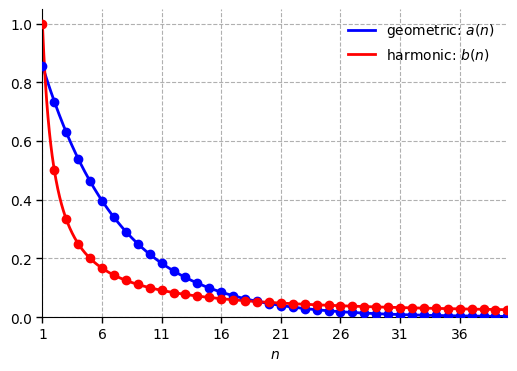
Consider an example geometric and harmonic series again:

The geometric series converges to zero faster, but it is hard to see if we plot each series as a function of $n$. The geometric is slower at first, and, by the time it catches the harmonic, both are already very small.

The same problem shows up anytime we want to compare the tails of a distribution. For example, if $X$ has power law tails, then we could have $p(x) \propto x^{-\gamma}$ for any $\gamma > 1$. Does $x^{-2}$ converge faster or slower than $x^{-3}$? How does the tail decay rate depend on the power of the power law, $\gamma$?

Once again, a plot is not too helpful, since the action is all squeezed to close to zero for the eye to discern.

For specificity, let’s focus on three power law type sequences:

It shouldn’t be too susrprising that the larger the negative power, the faster the sequence decays. Here’s a table comparing values for inputs spaced as powers of ten.

Notice that the last sequence converges much faster than the first. The first sequence adds one zero before the “1” each time we increase $n$ by a factor of ten. The second adds two zeros per factor of ten. The third adds three zeros per factor of ten. Notice, the number of zeros added matches the power of the power law.

Let’s write the table again, this time using scientific notation:

Finally, only report the exponents by changing the header from $n$, to $\log_{10}(n)$ and from the sequence values to the $\log_{10}$ of the sequence values:

Converting to a log scale on the input and output makes it much easier to compare rates of convergence. Here’s a corresponding plot using a log scale on both the input and output axes.

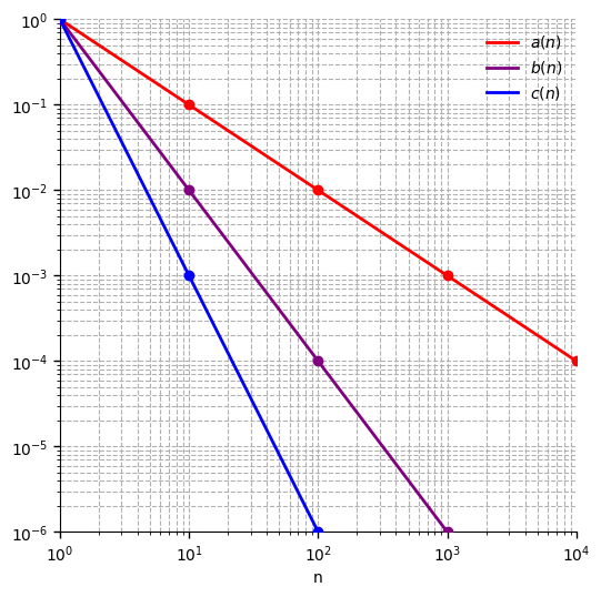
Notice, on the log-log plot, the power laws have become lines, whose slopes match their powers. The larger the negative power, the steeper the line on the log-log plot.

Log-log plots are very helpful tools for distinguishing rates of convergence. They are a good choice for visualizing tail decay since they convert power laws to lines, whose slope equals the power of the power line.

Comparing Asymptotic Rates¶

Formally, we can compare the rate at which two sequences do to zero as follows:

For example, $n^{-2}$ converges faster than $n^{-1}$ since $n^{-2}/n^{-1} = n^{-1}$ and $n^{-1}$ converges to zero as $n$ diverges.

Less trivially, consider the example sequences:

Taking their ratio:

Then, we want to find the value of the limit:

There are two ways to evaluate this limit. First, try simplifying. Divide the top and the bottom by $n^2$:

Alternately, recognize that $n^2$ diverges faster than $n$, so for large $n$ the $n^2$ terms will dominate. For example, when $n = 100$:

So, since the $n^2$ terms dominate, we can simplify by dropping all smaller terms:

So, in this case $a(n)$ and $b(n)$ converge to zero at the same rate.

For example, the sequence $a(n) = n/(1 + n^2)$ goes to zero as fast as $1/n$, so $a(n) = \mathcal{O}(n^{-1})$.

Anytime you are given a rational function for $a(n)$, you can identify its order of convergence by stripping out everything except the dominating term in the numerator and denominator. These are the terms where $n$ is raised to the largest power.

For example, the sequence:

If you can’t simplify the limit directly, or by stripping out everything but the dominating terms, then try using L’Hopital’s rule.

Consider the sequences:

for some integer $m > 0$. Which converges faster?

Let $f(x) = x^m$ and $g(x) = e^x$. Then we can apply L’Hopital’s rule to work out the limit.

1. If $m = 1$:

   $$L = \lim_{x \rightarrow \infty} \frac{x}{e^x} = \lim_{x \rightarrow \infty} \frac{\frac{d}{dx}x}{\frac{d}{dx}e^x} = \lim_{x \rightarrow \infty} \frac{1}{e^x} = 0.$$

   (19)

   So, $e^{-n}$ converges faster than $n^{-1}$. That’s not surprising. Exponential sequences adecay quickly, while harmonic sequences decay slowly.

2. If $m = 2$:

   $$L = \lim_{x \rightarrow \infty} \frac{x^2}{e^x} = \lim_{x \rightarrow \infty} \frac{\frac{d}{dx}x^2}{\frac{d}{dx}e^x} = \lim_{x \rightarrow \infty} \frac{2x}{e^x} = 0$$

   (20)

   since we’ve already shown that $\lim_{x \rightarrow \infty} x/e^x = 0$.

   So, $e^{-n}$ also converges faster than $n^{-2}$.

3. If $m = 3$:

   $$L = \lim_{x \rightarrow \infty} \frac{x^3}{e^x} = \lim_{x \rightarrow \infty} \frac{\frac{d}{dx}x^3}{\frac{d}{dx}e^x} = \lim_{x \rightarrow \infty} \frac{3x^2}{e^x} = 0$$

   (21)

   since we’ve already shown that $\lim_{x \rightarrow \infty} x^2/e^x = 0$.

   So, $e^{-n}$ also converges fatser than $n^{-3}$.

Repeating this argument inductively yields the following conclusion:

This rule generalizes our observation about geometric and harmonic sequences. The geometric sequence deacys exponentially, so decays faster than any power law. A distribution with exponential tails will have “lighter” tails than any distribution with power law tails.

The plot below compares the exponential function $e^{-(n-1)}$ to the power laws we plotted before.

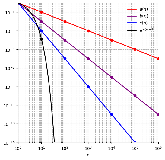
The exponential clearly converges faster than $n^{-1}$, $n^{-2}$, or $n^{-3}$. It converges faster than $n^{-\gamma}$ for any $\gamma > 0$ since the power law, $n^{-\gamma}$ would be a line with slope $-\gamma$ on the log-log plot, while the exponential is a concave curve whose slope grows steeper as $\log(n)$ increases on the log-log plot. No matter what $\gamma$ you choose, I could pick an $n$ large enough so that the exponential curve is decreasing faster than $-\gamma$.

Ordering Tail Decay Rates¶

During this week you will practice ordering sequences by their decay rates. We’ve set up some essential references in this chapter.

Our slowest example is the harmonic sequence, $n^{-1}$, which converges so slowly that its associated series, $\sum_{n = 1}^{\infty} n^{-1}$ diverges.

Our fastest examples are exponential/geometric, $r^n$ for $0 < r < 1$.

Power laws of the form $n^{-\gamma}$ for $\gamma > 1$ fall in between. They are faster than harmonic, but slower than exponential. They are ordered by their power.

Whenever you are given a distribution function, it is a good idea to check the tails, and to try and determine the order of convergence of the tail to zero. In essence, try to match its decay rate to the decay rate of some simple reference function (e.g. a power law or an exponential).