Section 1.3 and 1.4 establish rules for “not”, “or”, and “and” statements. However, we didn’t really finish the job for “and” statements. We showed how to organize joint probabilities, and how to use the rules for “or” to relate joints and marginals, but we didn’t derive any new rules that help us compute joint probabilities directly. We didn’t answer the question, how is related to and ?
In this section we’ll see that, to work out the probability that and happen, it is easier to first work out the probability that happens if happens (or visa versa). The probability that happens if happens is a conditional probability. We call it a conditional probability since the statement conditions on some other outcome, i.e. adds an additional condition that restricts the outcome space.
If Statements and Conditional Probability
What is the probability that it rains tomorrow if the weather is cold?
Suppose that:
| Event | Rain | Clouds | Sun | Marginals |
|---|---|---|---|---|
| Cold | ||||
| Warm | 0 | |||
| Hot | 0 | |||
| Marginals | 1 |
Then, when we condition on the assumption that it is cold, we are rejecting the possibility that it is warm or hot. In essence, we are restricting our outcome space. If it is cold, then it cannot be warm or hot, so any event in the sets “warm” or “hot” is not possible after conditioning. So, we can drop the bottom two rows of the table:
| Event | Rain | Clouds | Sun | Marginals |
|---|---|---|---|---|
| Cold |
Unlike the operations “not”, “or”, and “and”, which act on the definition of the event, the logical operation “if” acts on the space of possible outcomes, . So, unlike the first three operations, which change the composition of the event, “if” changes the list of outcomes that could occur. As a result, conditioning will change both the numerator and the denominator when we equate probability to proportion or frequency. All other operations only act on the numerator.
Normalization
Take a look at the conditioned table. All of the numbers in the table are nonnegative and less than one, so could be chances, however, they don’t add to one, so fail to form a distribution. The marginal, at the far right, is , not 1, so the list can’t define a full distribution.
There’s an easy fix here. The list of joints add to , so, if we scale them all by , they’ll add to 1:
So, we can get a valid distribution if we rescale the joint entries of the row by its sum. This is the same as putting all elements of the row over the least common multiple of their numerators, ignoring the denominator, then replacing it with the sum of the numerators:
The same operation will work for any list of nonnegative numbers with a finite sum. If we have a list where for all , then:
is a valid categorical distribution. This operation is called normalization since it rescales the entries to make sure they are normalized (add to 1).
Conditional Probability
When Outcomes are Equally Likely
While we could normalize our list to make a valid categorical distribution, it is not clear that we should. Why would normalizing by the marginal correctly return the conditional probabilities?
To answer this question we need a probability model that directs our calculation. Without a model, we could define conditional probabilities however we like. With a model, conditional probabilities have to behave in a sensible way.
Our first probability model is probability as proportion. If all outcomes are equally likely, then the probability of an event is the number of ways it can occur divided by the number of possible outcomes. In other words, the probability of an event is the proportion of the outcome space contained in the event. We can use this model to define conditional probability for equally likely events.
Think again about what “if” does to our model. When we condition, we are restricting the set of possible outcomes. For instance, in the weather example, we reject all outcomes where the temperature is warm or hot. If we roll a die, and condition on an even roll, then we are rejecting all odd outcomes.
Since we have a rule that assigns chances to outcomes when the outcomes are equally likely, we can compute conditional probabilities using this rule:
The probability a fair die lands on a 2 given that the roll is even:
The probability a fair die lands on a 2 or 4 given that the roll is even:
The probability a fair die roll is less than 3 given that the roll is even:
The probability a fair die roll is equal to 3 given that the roll is even:
In other words, the conditional probability of an event given another event , when outcomes are equally likely is:
We can rewrite the equation to recover the normalization rule we suggested earlier:
So, when outcomes are equally likely, we can compute conditional probabilities by isolating all outcomes that are consistent with the conditioning statement, then matching probability to proportion in the restricted space. In other words, just normalize the necessary collection of probabilities.
By Diagram
Here’s a visual argument. When outcomes are equally likely chances are proportions. We can make this analogy visual by drawing Venn diagrams, and computing the size of a set using its area in the diagram. This idea will come back formally in Section 2.3. You should remember that this is just a visual analogy. However, its useful since all of the rules of probability match the rules for proportions of area.
Here’s the Venn diagram representing given .
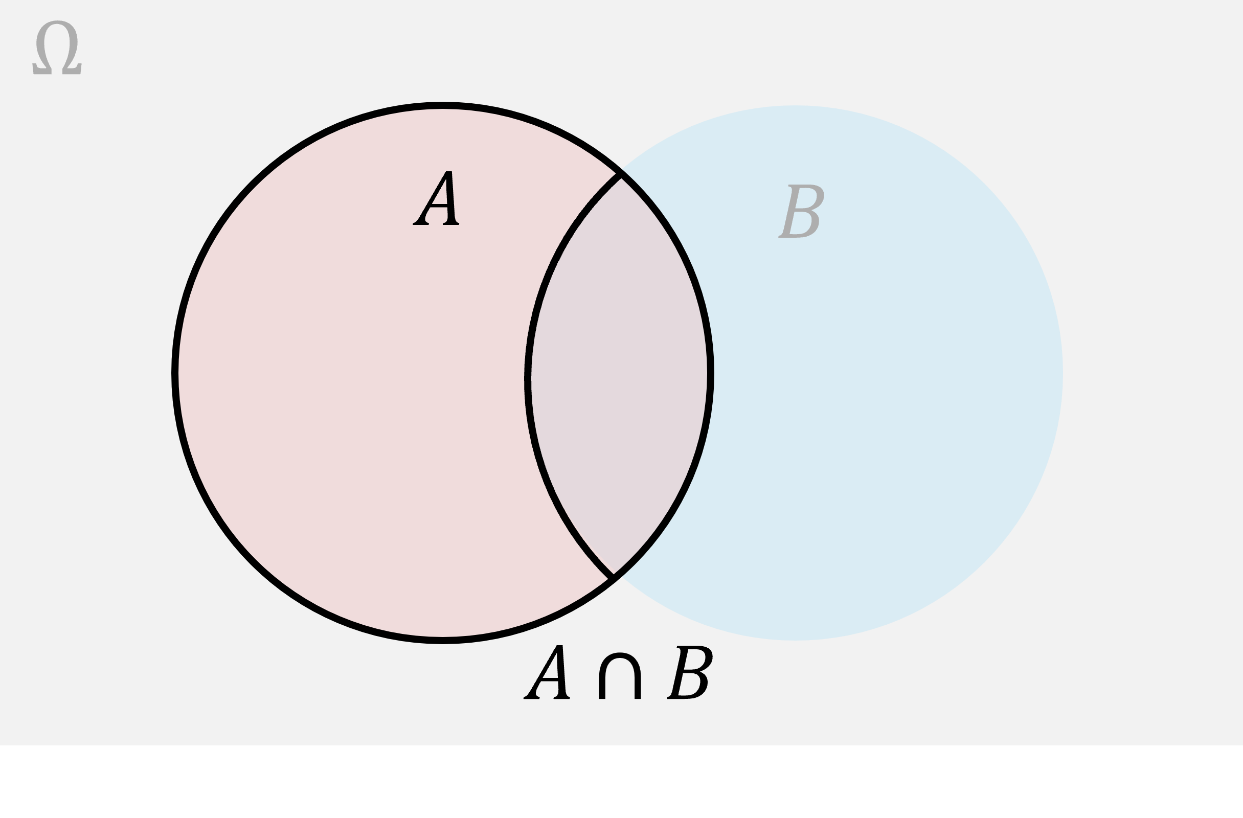
As usual, when we condition on an event we restrict our attention to only the outcomes consistent with that event. So, we’ve grayed out the whole diagram outside . All of the outcomes where happens, assuming we start in , lie in the intersection . So, using probability by proportion, the chance of given should be the ratio of the area of the intersection, to the area of :
In other words, the percent of the area of that is in both and is the percent of in both and , divided by the percent of in . That’s the division rule we proposed for conditionals.
This vidsual is helpful since it highlights a potential disparity that confuses many students.
If and are different sizes (e.g. is much more likely to happen than ) then the percent of in the intersection will not equal the percent of in the intersection. Since and are different sizes, but share the same intersection, for a fixed intersection, more of will be in the intersection than .
Here’s a matching diagram for :
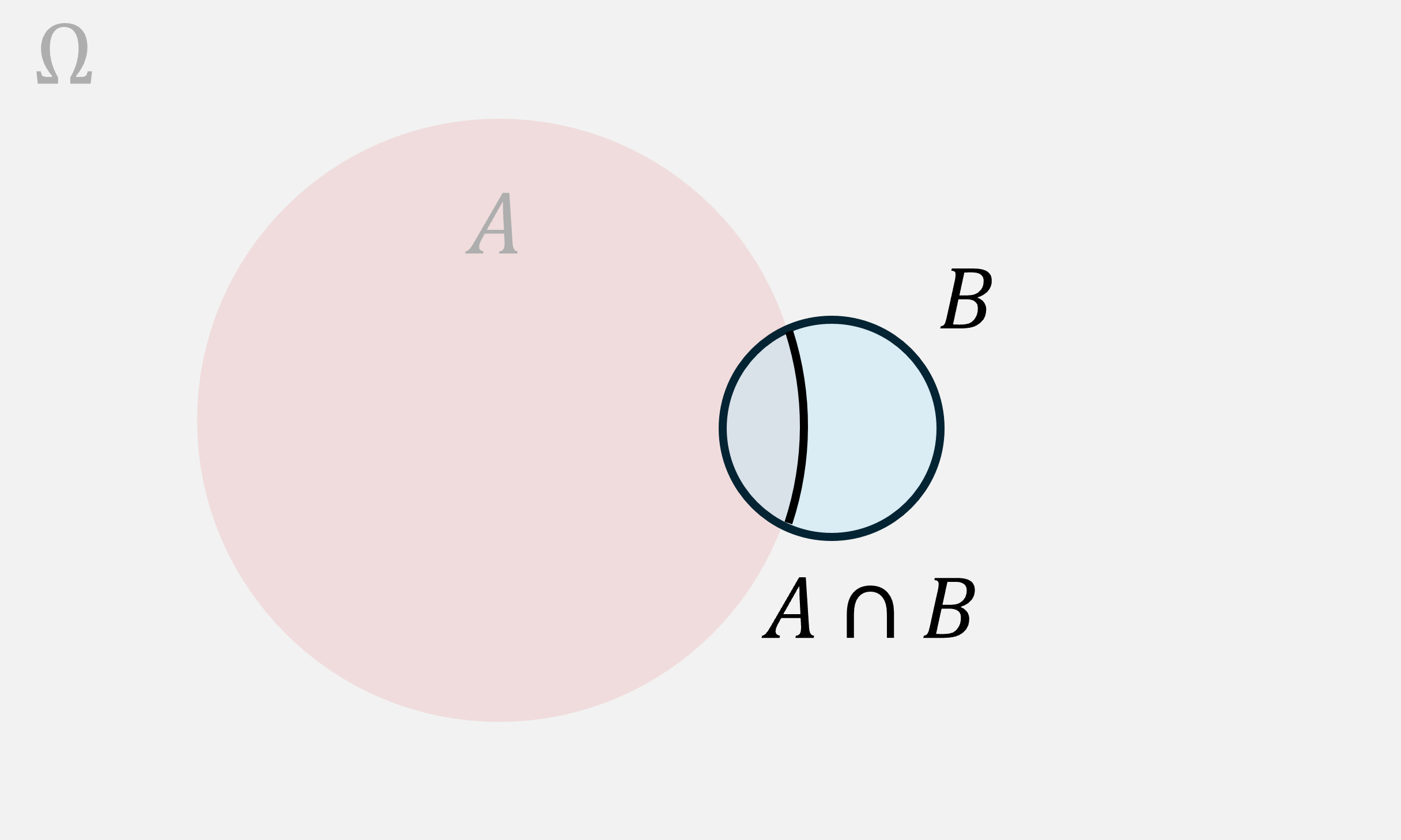
Notice that, in this case, about a third of is in the intersection. If we’d asked for the chance of given we’d have gotten about .
On the other hand, since is much bigger than , only a small percentage of is in the intersection. Maybe one tenth. Then, if we’d asked for the chance of given , we’d have gotten about . These numbers are different. They can be radically different. They share the same numerator (the size of the intersection or joint), but can have totally different denominators. As a result and will differ dramatically when the marginals, and , differ dramatically. We’ll walk through a dramatic applied example at the end of this section.
Does the rule work if the underlying outcomes are not equally likely?
Consider our weather example again. We can isolate the appropriate row of the joint table:
| Event | Rain | Clouds | Sun | Marginals |
|---|---|---|---|---|
| Cold |
but we don’t know anything about the background outcome space that produced these joint probabilities. Moreover, trying to spell out a detailed weather model in which all microscopic outcomes are equally likely is both far too much work for this problem and would be impractical in almost all settings. For conditional probability to be useful, we should be able to compute it in categorical settings, without somehow expanding our outcome space. So, while the derivation provided above works for equally likely outcome models, it is too restricted to work for general applications.
By Conditional Frequency
Thankfully, we have at hand an alternate model; probability as frequency. Recall that, the probability an event occurs should be approximated by, and equal in the long run, the frequency with which it occurs in a sequence of repeated trials. This relation should hold for any valid probability model. So, let’s use it to show that the normalization approach correctly computes conditional probabilities.
Consider a long weather record. Say, the weather in Berkeley over the last year. Let’s try to find the conditional probability that it is cold, and rains, on some future day selected at random. We’ll assume that the climate is fixed, the process that produces weather does not change (is stationary), and the process doesn’t remember its past forever (e.g. the probability that it rains today given that it rained on this day a century ago is the same as the probability that it rains today). Then the probability of any event should be approximated by the frequency with which the event occurs in the weather record.
To keep our record short we’ll use the following visuals:
| Event | Rain | Clouds | Sun | Cold | Warm | Hot |
|---|---|---|---|---|---|---|
| Precip. | 💧 | ☁️ | ☀️ | 🥶 | 😎 | 🥵 |
| Symbol | R | Cl | S | Co | W | H |
Here’s an example two-week record:
| Day | 1 | 2 | 3 | 4 | 5 | 6 | 7 | 8 | 9 | 10 | 11 | 12 | 13 | 14 |
|---|---|---|---|---|---|---|---|---|---|---|---|---|---|---|
| Precip. | 💧 | ☁️ | ☁️ | ☁️ | ☀️ | ☀️ | ☁️ | 💧 | 💧 | ☁️ | ☀️ | ☀️ | ☀️ | ☁️ |
| Temp | 🥶 | 🥶 | 🥶 | 😎 | 😎 | 🥵 | 😎 | 😎 | 🥶 | 🥶 | 😎 | 🥵 | 🥵 | 😎 |
We can compute frequencies from this record. For example and since it rained on 3 days, and was cloudy on 6, out of the last 14.
We can also use this record to compute joint frequencies. For example since it was rainy and cold on 2 of the 14 days. These were days 1 and 9.
Here’s the good part. We can also compute conditional frequencies from the record. Suppose I wanted to find the frequency with which it rained, given that it was cold. Then, I would disregard all days when it wasn’t cold, and compute the frequency out of the remaining days. Disregarding the days when it was not cold is equivalent to filtering for only the days when it was cold:
| Day | 1 | 2 | 3 | 9 | 10 |
|---|---|---|---|---|---|
| Precip. | 💧 | ☁️ | ☁️ | 💧 | ☁️ |
| Temp | 🥶 | 🥶 | 🥶 | 🥶 | 🥶 |
Now that we’ve filtered the record for only cold days, the conditional frequencies are apparent:
since it rained on 2 of the 5 days when it was cold. Notice, 2/5 = 0.2 is not a bad estimate to the value we got by normalizing, . These two numbers are different because our record of cold days was short, so the frequencies are only rough estimates to the true probabilities.
Nevertheless, the algebra for conditional frequencies is clear, and, should recover the appropriate probabilities if we run enough trials/collect a long enough record.
Take a look at the frequency calculation again:
This expression looks a lot like what we wrote for equally likely outcomes. All we’ve done is changed the way we count. Instead of counting ways an outcome can occur, we are counting the number of times it did occur in a sequence.
Let be the number of times it rained and was cold (2), and be the number of times it was cold (5). Let be the length of the record (14). Then:
Compare these statement to what we wrote for equally likely outcomes. They are identical, up to substituting frequency for probability. Since frequencies should match probabilities on long trials (in the limit as goes to infinity), we’ve just derived the general definition for conditional probability:
In our example, exactly as we predicted by normalizing.
If we want probabilities to match long run frequencies, this is the only sensible definition. You should remember it, conditional equals joint over marginal.
Divide by the Appropriate Marginal
Always make sure that you divide by the marginal that matches the event you conditioned on. If you forget what to divide by, either:
Go back to the normalization argument and check that you divide by the quantity needed to normalize the conditional distribution.
Remember that we are filtering for only the outcomes that are consistent with the conditioning statement, so need to reduce the size of the outcome space, or length of the record, by the fraction of the outcome space/length of record that is consistent with the conditioning statement. We filtered for days when it was cold, not days when it rained, to find the conditional probability it rains when it is cold.
Conditioning Preserves Odds
The following sectional is optional. It suggests an axiomatic method for deriving the conditional probability formula by requiring that relative chances are unchanged by conditioning.
Equating Odds
The definition, conditional equals joint over marginal, can be justified without referencing frequencies. We can, instead, generalize the rule we introduced for equally likely outcomes. We said before that, if two outcomes are equally likely before conditioning, then, if both outcomes are consistent with the conditioning statement, they should be equally likely after conditioning.
More generally, we might require that the relative likelihood of two outcomes is unchanged by conditioning if both outcomes are consistent with the conditioning statement. For instance, if it is twice as likely to rain and be cold than to be sunny and be cold, we should expect that it is twice as likely to rain if it is cold than to be sunny if it is cold.
The argument provided above is a statement about odds. The odds of two events is a comparison of their likelihood. Specifically, the odds happens relative to is defined:
So, if then is twice as likely as .
It turns out that, if we know all of the odds for a set of outcomes, then we also know their probabilities. For instance, suppose that there are three possible outcomes, and is twice as likely as and three times as likely as . Then the list of their probabilities must be proportional to the list . This is a list of nonnegative numbers, so there is only one matching distribution. The only matching distribution is the distribution we recover by normalizing:
So, knowing the odds is the same thing as knowing the distribution.
If the relative likelihood of two events that are consistent with the condition is unchanged by conditioning, then it must be true that conditional distributions are recovered from joint distributions by:
isolating the appropriate row or column of the joint probability table
dividing all joint entries by their sum, which is the associated marginal
Conditional Distributions
Let’s practice using this rule. Here’s the weather example again:
Write down the joint table:
| Event | Rain | Clouds | Sun | Marginals |
|---|---|---|---|---|
| Cold | ||||
| Warm | 0 | |||
| Hot | 0 | |||
| Marginals | 1 |
Filter for only the cold events:
| Event | Rain | Clouds | Sun | Marginals |
|---|---|---|---|---|
| Cold |
Normalize by the marginal:
| Event | Rain | Clouds | Sun |
|---|---|---|---|
| Cold |
Notice that the conditional distribution is proportional to the list of joint probabilities in the isolated row. This is a nice visual rule of thumb. If you have a joint table, and want the conditionals, just look up the appropriate row or column and scale it.
For instance, if we conditioned on sun, we’d isolate the column:
| Event | Sun |
|---|---|
| Cold | |
| Warm | |
| Hot | |
| Marginals |
Then rescale to find the conditional probabilities:
| Event | Sun |
|---|---|
| Cold | |
| Warm | |
| Hot |
The Multiplication Rule
Now that we know how to handle “if” statements, we can go back to our original aim, understanding “and” statements. Consider the definition of a conditional probability:
Rearranging the expression gives our next fundamental probability rule:
This rule is sensible. Suppose that four in every ten days are sunny, and half of all sunny days are hot. Then it is sensible that the fraction of all days that are both hot and sunny should equal the fraction of all days that are sunny, times the fraction of all sunny days that are hot. This is precisely the calculation we performed to find the probability that a sunny day is hot in reverse:
The multiplication rule should be used in the same fashion as the addition rule or the complement rule. Use it if:
You are asked for the probability of some event,
that event is naturally expressed as a joint event or intersection (it can be expanded as a sequence of “and” statements) where,
the individual parts are each simpler to work with.
In particular, look for examples where the event is best described with a conditional sequence. Then you can find the joint probability by simply walking through the sequence.
Example
Consider, for example, the probability that we draw two aces in a row, when we draw two cards from a thoroughly shuffled deck. We worked this probability out by counting in Section 1.2. There, we computed:
We noticed that the 50! term cancelled because the order of the last 50 cards in the deck didn’t matter, but, we didn’t have an organized way of calculating this probability without counting the number of two card hands that are a pair of aces, relative to the number of possible two card hands.
Notice that:
These numbers are suggestive. There are four aces in the deck of 52. After removing an ace, there are three remaining in a deck of 51. So:
Therefore:
In short, the chance we draw two aces in a row is the chance our first draw is an ace, times the chance our second draw is an ace if our first draw was an ace.
If you’ve used the multiplication rule before, this approach might have seemed the most natural to you. Now we know why it is true. Anytime you are inclined to describe an event with a conditional sequence (first happens, then happens, then happens, ...) you should try the multiplication rule.
Notice: ⚠️ the multiplication rule does not tell you to directly multiply marginal probabilities. This is a common mistake. Always multiply a marginal with a conditional. Otherwise, your calculation will be incorrect. In the example above, the chance of drawing an ace on the first draw is and on the second draw is , but the chance of drawing two aces is not .
Generalization
The multiplication rule generalizes naturally to longer sequences of events. The probability that and and happen is:
You should read the equation above, the probability that , , and all happen is the probability happenss times the probability happens if happens, times the probability happens if and both happen.
For a longer sequence, we get the chain rule:
We can now complete out summary table of probability rules:
Reasoning with Sequences
The multiplication rule, and its extension to sequences of events, gives us a new visual tool for computing probabilities.
Consider the weather example again. If we rewrite the table thinking first about the marginal chance of temperature, then the conditional chances of precipitation, we can express the probability model:
| Event | Marginal Probability |
|---|---|
| Cold | |
| Warm | |
| Hot |
and
| Event | Rain | Clouds | Sun |
|---|---|---|---|
| if Cold | |||
| if Warm | 0 | ||
| if Hot | 0 | 1 |
This information can be represented with an outcome tree. The outcome tree works like a decision tree. First ask, what is the temperature? Then ask, given the temperature, what is the precipitation? Label each edge in the decision tree with the matching marginal or conditional probability:
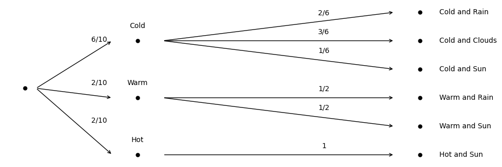
To find the joint probabilities of the events at the far end of the outcome tree, simply multiply the probabilities down the matching path.
For example:
If you consult the joint table in Section 1.4, you’ll find the same value.
Bayes Rule
How would we find the conditional probability that it is warm if it rains?
Notice that, the outcome diagram sketched above does not provide this conditional directly. Nor does the specification:
| Event | Marginal Probability |
|---|---|
| Cold | |
| Warm | |
| Hot |
and
| Event | Rain | Clouds | Sun |
|---|---|---|---|
| if Cold | |||
| if Warm | 0 | ||
| if Hot | 0 | 1 |
Nevertheless, we can always find the desired conditional by first solving for the appropriate joint and marginal, then scaling the joint by the marginal. In many ways, this procedure is the same as what we’ve done before, only we start with different information.
Suppose that we know and the conditionals given , and . How can we find ?
Well, let’s use our rules.
Always start from what you need to find. By definition:
Let’s find the joint probabilities. If we have a complete joint probability table then we can find any conditionals we want. To find the conditional probability of given we need the joint . We can find it by multiplying down the appropriate path in the outcome tree:
We now have two ways of expressing the joint. Both are valid applications of the multiplication rule:
We can compute the top line, and want the last term in the bottom line. Since the two lines return the same joint they are equal, and:
By assumption, we know all the values in the numerator. That leaves the denominator. The demoninator is a marginal, so we can always expand it as we did in Section 1.4:
Then, since both terms on the right hand side are joint probabilities, we can find them with the multiplication rule:
Putting the numerator and denominator together gives Baye’s rule:
It is usually more helpful to think about Baye’s rule in two stages. First, find all the joint probabilities by multiplying down the paths of the outcome tree that point to an event where occurs. Then, find the marginal probability that occurs by summing over the joint probabilities. Finally, take the ratio of joint to marginal that recovers the desired conditional.
Here are two examples:
Warm if Rainy
What is the chance it was warm if it rained?
Calculate the joint that appears in the numerator:
Find the necessary marginal:
Expand the marginal by partitioning, then apply the addition rule for disjoint sets:
Find each joint using the multiplication rule:
Therefore:
Apply the definition of conditional probability (plug in):
So, if it rained, then there is a 1/3 chance it was warm.
To check our answer, look up the column of the joint table where it rained:
| Event | Rain |
|---|---|
| Cold | |
| Warm | |
| Hot | 0 |
| Marginals |
Normalizing by the marginal produces the same calculation.
Reasoning by odds, it is twice as likely to be cold if it rains than warm if it rains, and it is never hot, so the chance it is warm, if it rains, is one third.
Ace On First Draw If Ace on Second
If I pull two cards from a thoroughly shuffled deck, and the second card was an ace, what is the chance the first card was an ace?
Before we solve this problem, take a moment to think about what knowing the second card was an ace should tell us about the first card. If we know nothing the probability the first card was an ace is since there are 4 aces in all 52 cards. However, if we pull an ace on the first draw, then we are less likely to draw an ace on our second draw. It stands to reason that, if we did draw an ace on our second draw, the chance we drew an ace first should be less than . Let’s check...
Calculate the joint that appears in the numerator:
Calculate the necessary marginal. In this case we can do it directly. Knowing nothing about the first draw, the chance we draw an ace on our second draw is :
Apply the definition of conditional probability (plug in):
Then, as expected . In other words, learning that the second draw is an ace decreases the chance the first draw was an ace.
Problems in the Philosophy of Chance
The second example shows something odd about conditional probability. If we draw cards in sequence, the possible second cards drawn depends on the outcome of the first draw, but the second card drawn cannot influence the first card drawn since it was drawn after the first. Yet, observing the second draw can change what we know about the first draw. While the second draw cannot influence the first draw in a causal way, it can change the conditional chance the first card was an ace.
This distinction between a causal relation, and an informational relation, may seem reasonable here, but it points to some of the deepest questions in probability. Is probability a model for information, and how we learn from evidence? If so, then there is no contradiction in the conditional statement that the we can gain information about the first card from the second. If instead, probability is a model for truly random events then we are in a pickle since, by the time we are drawing the second card, the first card must be drawn, so cannot be random. We might not know its value (imagine drawing it but leaving it face down), but it is either an ace or not. It is not random. You could even imagine asking a friend to draw both cards and tell you only the value of the second. Your friend knows whether the first card is an ace or not. How then can we discuss its conditional probability? Does it make sense to say the value of the first draw is random simply because you don’t know it?
These distinctions are an important part of the philosophical debate between two famous camps of statisticians, the Bayesians, who adopt probability as a self-consistent language for expressing uncertainty and for learning from information, and the Frequentists, who adopt a more restrictive definition that requires an empirical relation to frequency in a series of experiments. It also points to a thorny definition issue that we’ve glossed over... what do we mean when we say a process is random?
We’ll save this discussion for later. In the end, the more practical issue between the Frequentists and Bayesians regards uses and misuses of modeling anyways. If you are curious, come talk to the Professor.
Keep this example in mind when you work on the Monty Hall problem in your homework this week.
Example: Base Rate Neglect
Let’s look at a practical problem where the Bayesian approach is necessary.
Suppose you are subject to a medical test that is designed to determine whether or not you have some medical condition. For example, you take a Covid or Flu test. The result of the test is important, since it will impact your behavior. For example, if you are sick, you might decide to stay home, or may invest in a medical intervention which is costly.
No test is perfectly accurate. In essentially all cases a test could predict that a healthy patient is sick, or that a sick patient is healthy. Let denote the event that the recipient is healthy, the event they are sick, the event that the tests returns negative (predicts healthy), and the event that the test returns positive (predicts sick). Then, there are four possible outcomes. We can arrange them just like we did a joint probability table:
| Event | N | P |
|---|---|---|
| H | TN | FP |
| S | FN | TP |
Here the labels TN, TP, FN, FP stand for (true/false) and (positive/negative). Notice that there are two ways the test can make a mistake. Either it falsely predicts positive or falsely predicts negative. Both rates matter. False positives are costly and can be harmful to the recipient if they take actions assuming they are sick. At worst, a false positive can lead to uneccessary medical intervention. False negatives are dangerous, since the recipient may act as if they are healthy, so may risk others’ health, or not take medical action that could address their condition.
It is standard in test design to control the false positive rate. That is, the conditional probability that the test returns positive if the truth is negative (i.e. the patient is healthy). The smaller the false positive rate, the more significant the test result, and the more specific the procedure. The other error rate, the probability the test misses a sick patient, controls the power of the test (its ability to detect sick patients) and its sensitivity (how sensitive it is to evidence of disease).
Let’s name these probabilities:
Suppose that:
This looks like a good test. It is reasonably selective/specific, since it only makes a false detection for 5 percent of patients. It’s also pretty powerful/sensitive. It only misses a true detection in 1 percent of sick patients. For reference the significance of a mammogram is 90%, so about 10% of healthy women are falsely flagged for breast cancer. The sensitivity of mammograms is 87%, so they have a false negative probability of 0.13.
Now suppose you take the test, and it returns positive. Should you act as if you are sick? What is the probability you were a false positive, and are actually healthy? In other words, what is
Problems in the Philosophy of Chance
So far, we don’t have enough information to answer the question. We have the conditional probabilities of the test outcomes given the patient’s health, but not the conditional probabilities of the patient’s health given the test outcome. To find the conditional probability of the patient’s health given the test outcome, we need a joint probability model that can assign joint probabilities to every entry in the table. This means that we must model the pateint’s health as random.
Here again, we hit a philosophical snag. If we believe that people can be sick or healthy, then at any given time, an individual is sick or healthy. Whether they are sick or not is not determined randomly when they happen to take a test. So, while they may not know whether they are sick, there is a fixed ground truth answer. The idea that there is a fixed ground truth answer is baked into the “true”, “false” labels we used to describe the error rates.
Yet, we’re really asking a question about information and uncertainty. What should the patient learn from the test result, and how should they behave in response?
When we ask an informational question, it is reasonable to think that the patient should make decisions as if their unknown health status was random. This is not such a strange idea. Imagine that I roll a die inside a cup but keep the cup over the die. Once the die stops bouncing it has landed on a side, so its value is no longer random. Since it is covered, and we don’t know its value until we remove the cup, we’d be justified in treating the die’s value as if it were still random. This approach is especially well justified if we have to bet on multiple rolls, then reveals, of the covered die.
For an explicit example, imagine that you are not a patient, but are instead a doctor, or national health service, that applies the test and recommends action. You don’t apply the test once, you apply it many times. So, you want it to give accurate advice for most patients, e.g. on average.
When you try to make decisions that work, on average, over a population, you could model the situation by imagining that the decisions are applied to a randomly selected sample of individuals. From the doctor’s perspective it is quite sensible to imagine that a patient’s true health status is a random quantity, since they could imagine applying the test after selecting a random sample of patients. As long as the frequency of sick individuals in their sampling model matches the actual frequencies of patients who the test is administered to, then the doctor’s decision to model the process that sends her patients as random won’t lead her to make any errors that are based on averages expressed as chances.
Imagine that, of all patients who take the test, percent are actually sick. This percent is sometimes called a base rate. Base rates can influence conditional chances in surprising ways.
In many settings, they are quite small. For example, only 0.5% of women screened for breast cancer in a mammogram are diagnozed for breast cancer in a follow up test. Since the mammogram is meant to filter for women with breast cancer, the population screened post mammogram should include more cases of breast cancer, so should have a higher base rate than the population of all women who take the mammogram. So, let’s be conservative, and assume that the second stage test is perfect. Then we can put a conservative upper bound on the base rate of cancer in the population of women undergoing the mammogram at .
Using Outcome Trees
Here’s an outcome tree representing the test, labelling the marginal probability for each test outcome:
We could compute any of the joint probabilities for any of the outcomes by applying the multiplication rule. For example, the chance of a true negative outcome is . In other words, of all women who get a mammography, 89.55% should be healthy and receive a negative test result (the test predicts healthy). Alternately, the chance a woman is healthy, but receives a falsely positive test result, if . In other words, 9.95% of women will be healthy but incorrectly flagged as positive. Nine percent is a lot of women, but it is not too large given the test accuracy. So far, the test looks reliable.
However, the diagram does not match our question. We didn’t ask what is the chance a woman is healthy and is falsely flagged as sick? The woman’s health status is unknown. The entire premise of the test is that we can’t know her health status, and that the test might be wrong, but is usually right. We asked, what is the chance a woman is healthy if she is flagged as sick. Notice that we’ve only conditioned on what we could observe, then asked a probability question about what we can’t observe.
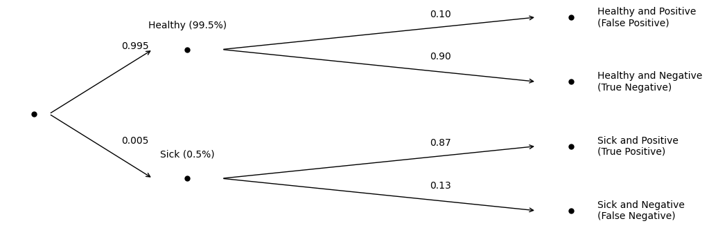
Since we can’t observe a woman’s true health status, we should really draw the diagram in a way that groups all outcomes where the test result is identical:
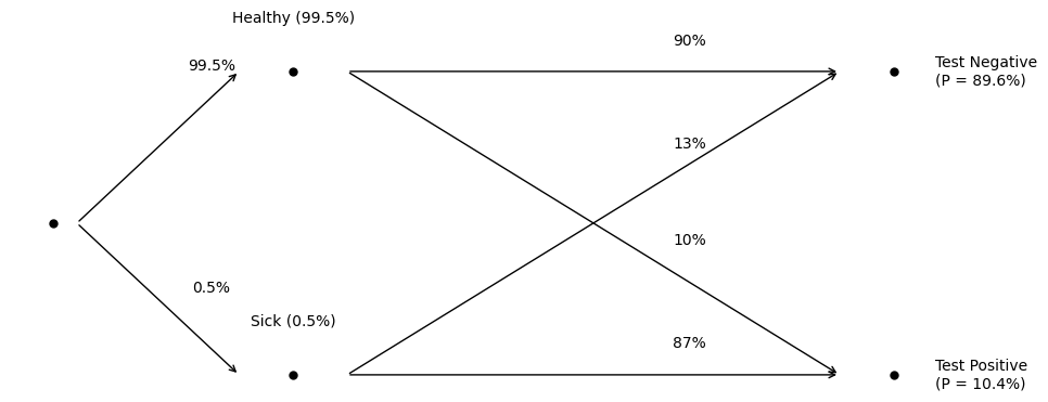
Notice how the arrows corresponding to test decisions have moved. The arrows that move straight across are true predictions. The arrows that cross are errors. The error chances are relatively small since the test rarely makes a mistake when we condition on the patient’s health status. When we ask, what’s the chance a woman flagged as sick is healthy, we asked what percent of the positive cases come from the diagonal error arrow.
Take a look at the marginals. Something odd has happened. Compare the marginal fractions of woman that are actually sick (0.5%) to the number that have been flagged as sick (10.4%). Almost 20 times as many women have been flagged as sick than women who are actually sick! So, most of the women flagged as sick must be healthy!
By Population Diagram
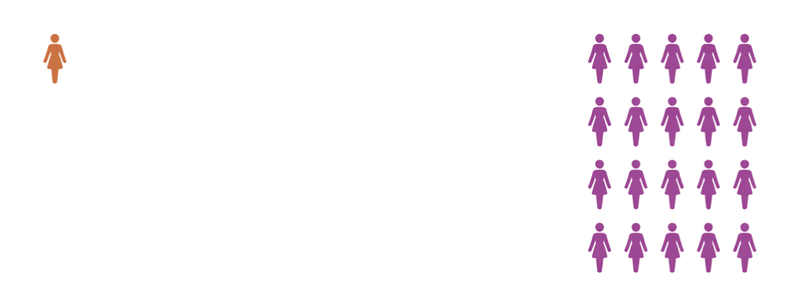
Let’s try this a bit more directly. Here’s a grid of 200 women. You can imagine that each icon represents 100 women who get tested each year, so this grid represents a population of 20,000 women. The base rate is 0.005, so we’d expect women in this population to be sick. We can represent those women with one icon.
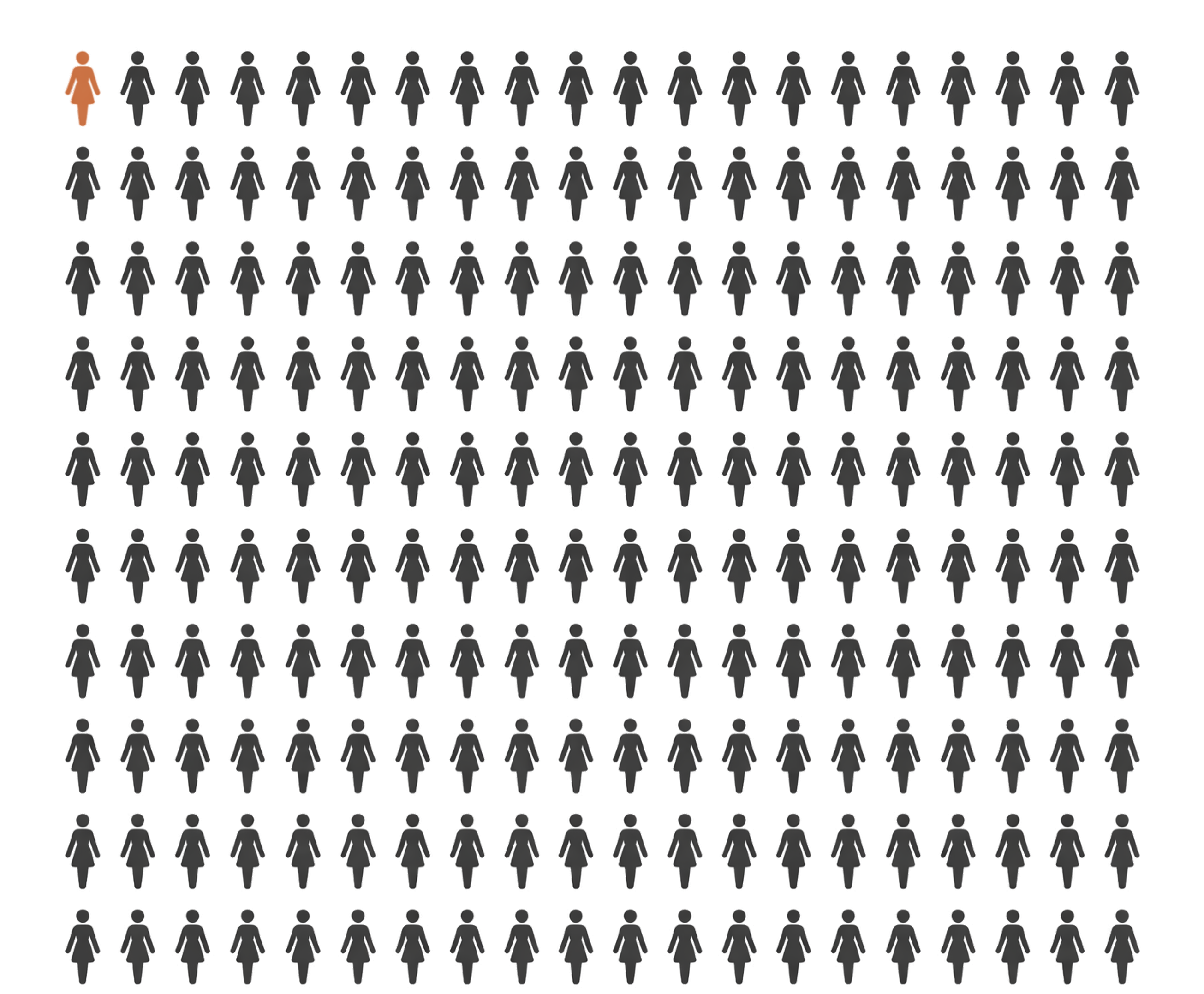
All the grey icons are healthy. The one orange icon represents the sick women.
What fraction of the healthy women get incorrectly flagged as sick? Well, the chance of a false positive was 0.10, so 10% of the remaining 19,900 women will be flagged. Thats 19.9 icons, so 20 icons. We’ll represent these women with purple.
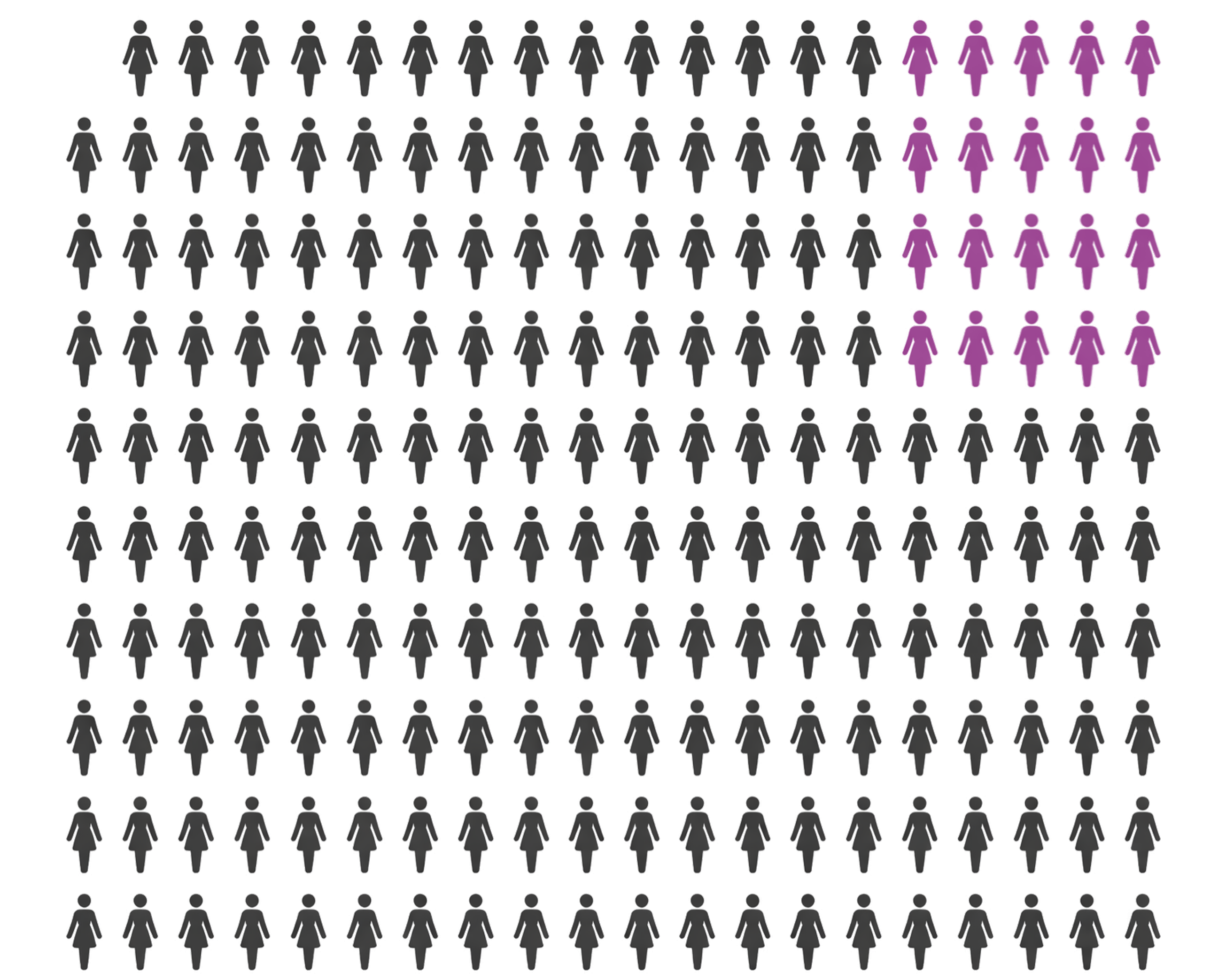
Most of these cases are correctly diagnosed as healthy. Why the high error rate the other way around?
Most of the sick women get detected, so we can be optimistic and assume all of those women get detected. So, here’s the whole population with all the sick women highlighted and all the false positive cases highlighted:
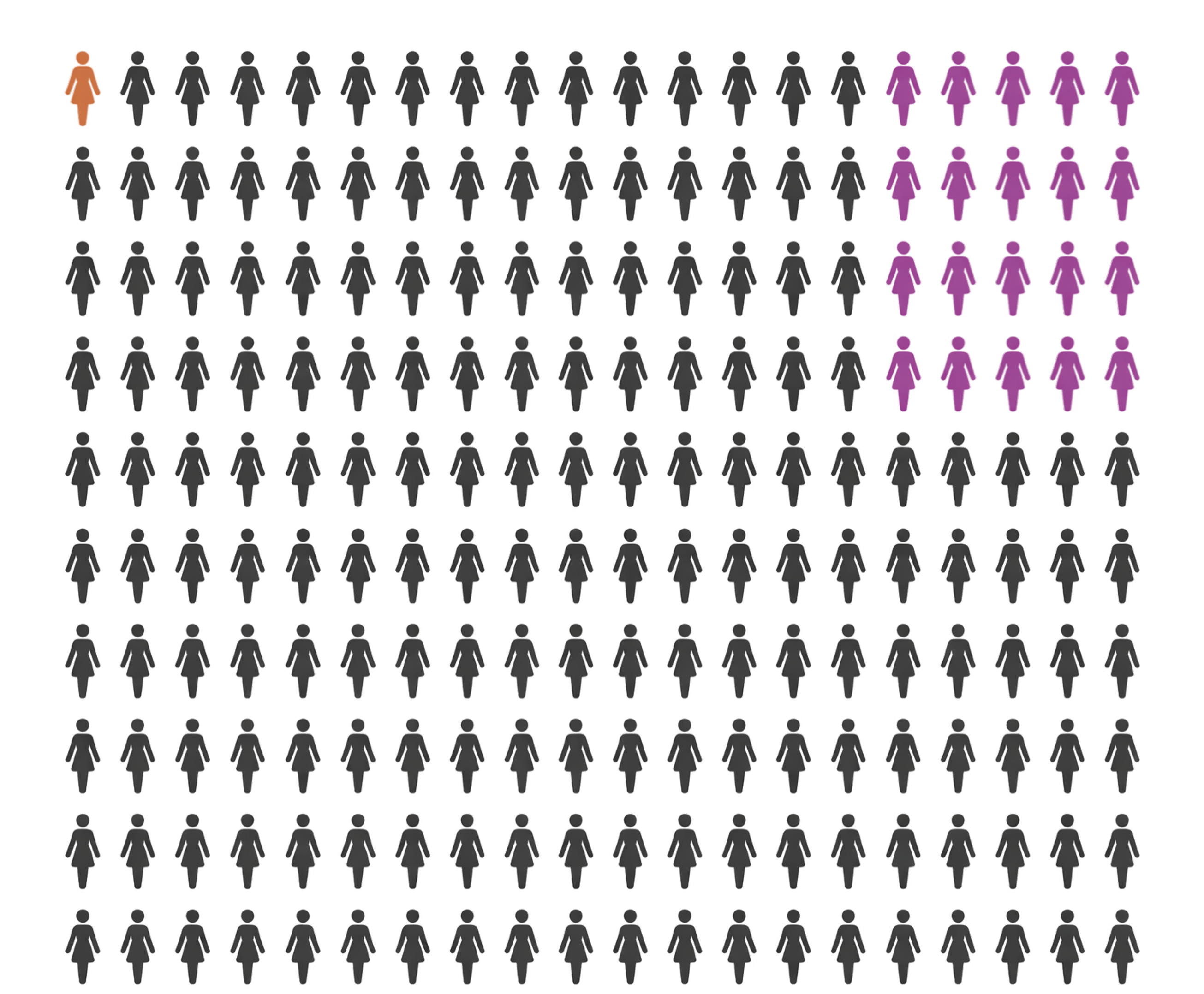
Then, filtering for only the positive cases, we can see the issue:
Most of the positive cases are false positives since the base rate is so low. 100% of a small population is smaller than 10% of a much larger population.
Let’s compute a lower bound on the chance a woman who recieves a positive mammogram does not have breast cancer via Bayes rule:
That’s a shocking number. Read it again. Don’t skim it.
Even though only 10% of healthy women get flagged by the mammogram, then the fraction of women flagged by the mammogram who actually have breast cancer is at least 95%!
Pause to let that sink in. What’s happened here?
The problem is the base rate. The base rate of actual sick cases is so low that, even with a reasonably accurate test, the small fraction of healthy cases who are flagged as sick vastly outweighs the large fraction actually sick cases who are flagged as sick. Why? Because there are 995 healthy cases for every 5 sick cases.
What about our hypothetical test with and . This is a much more accurate test. Can it filter out enough healthy cases so that a patient who receives a positive result is usually sick?
Even with the better test, the chance that a patient who received a positive result is actually healthy is still greater than 90%.
This is why we should use multistage test procedures when false positives are a problem, and base rates are low. Forgetting to account for the base rate is sometimes called base rate neglect.