8.1 Coordinate Systems

To extend our modeling framework to multiple dimensions we will need to introduce language for describing mutlivariate problems. The most basic component of that language is a coordinate system.

Coordinate systems assign locations in a space to lists of numbers. Each number in that list is a coordinate. Distinct coordinates convey different information about the location of the point specified by the coordinates.

Consider a plane. Points on the plane can be described by:

1. Fixing an origin and two perpendicular axes. Then, measure the distance from the point to the origin on each axis. Call these numbers $x_1$ and $x_2$. Then each pair $[x_1,x_2]$ identifies a point in the plane that is $x_1$ units away from the origin along the first axis, and $x_2$ units away from the origin along the second axis. This is a Cartesian coordinate system.

   

   • For instance, imagine that you are at a rectangular desk. Place a point in the center of the desk. Align one axis to run straight away from you. This is the front-back axis. Then, align the other axis to run perpendicular to the first axis. This is the left-right axis. Then, a point $[1.5,-0.2]$ is a location 1.5 units back, and 0.2 units left of center. Notice that the axes must be oriented. We had to choose that +1.5 meant motion backward, not motion forward, and that -0.2 meant motion left, not right.

   • Imagine you are given a rectangular piece of graph paper. Place a dot on one of the corners in the graph paper. Call this the origin. Then each other corner in the grid can be represented with a pair of numbers, $[x_1,x_2]$ corresponding to the distance up, and the distance across, from the origin.

   • Cartesian coordinates generalize easily to higher dimensional spaces. For instance, in three-dimensions, we can specify locations by measuring a distance out, across, and up, from an origin.

2. Fix an origin and one ray leaving the origin. Then, for any point, draw a line segment from the origin to the point. Measure the length of the line segment, and the angle between the line segment and your reference ray. Now each pair, $[r,\theta]$ represents a point on the plane. This is a polar coordinate system.

   

   • By convention, the first polar coordinate is usually denoted $r$ for “radius.” It is the radius of a circle, centered at the origin, passing through the point of interest.

   • By convention, the first polar coordinate is usually denoted $\theta$ for “angle.” Sometimes we denote angles with $\phi$, or, less frequently, $\psi$.

In both cases we started by fixing an origin. The origin of a coordinate system is the location assigned coordinates $[0,0]$.

Coordinate systems assign points in a space to lists of numbers. Since distinct coordinates encode distinct information, their order matters, and we usually fix a convention for their order. For instance, in polar coordinates, it is standard practice to list the radius before the angle.

Vectors¶

Finitely long, ordered lists of numbers are vectors.

For example, $v = [v_1,v_2]$ is a two-dimensional vector with entries $v_1$ and $v_2$. If it is unclear whether $v$ is a vector, then we might use the notation $\vec{v}$ to emphasize that $\vec{v}$ is a vector.

Often, vectors are interpreted as arrows, emanating from the origin, and terminating at the point in a Cartesian coordinate system with coordinates equal to the entries of the vector. For example, the vector $[2,5]$ is the arrows starting at the origin, $[0,0]$ and ending 2 units across and 5 units up from the origin. The vector $[4,-1]$ is the arrow starting at the origin, $[0,0]$, and ending 4 units across and 1 unit down from the origin.

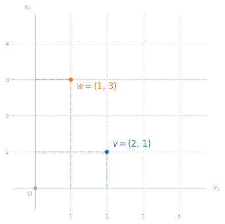
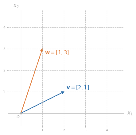
Here are two example vectors:

In other words, a random vector is just a collection of random numbers.

Vector Operations¶

We can do algebra with vectors just like we can do algebra with numbers. The algebra of vectors is the subject of linear algebra. We will only need the essentials.

Vector Addition¶

For example:

We can draw this new vector using the tip-to-tail rule. Starting from the origin, move to the location $v$. Then, from $v$, move to $v + w$ by translating the arrow $w$ so that it starts from $v$ instead of from the origin.

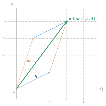
Alternately, draw a parallelogram with a corner at the origin, and sides parallel to $v$ and $w$. The missing corner is $v + w$.

Like scalar addition, vector addition is commutative and associative so:

Scalar Vector Multiplication¶

It is common practice to denote scalars with greek letters (e.g. $\lambda$) and vectors with roman letters (e.g. $x$, $y$, $v$). Sometimes scalars are represented with roman letters drawn from the start of the alphabet (e.g. $a$, $b$, $c$).

For example, if $\lambda = 3$ and $v = [1,-2]$ then:

The result is new vector, parallel to the original vector, but three times longer.

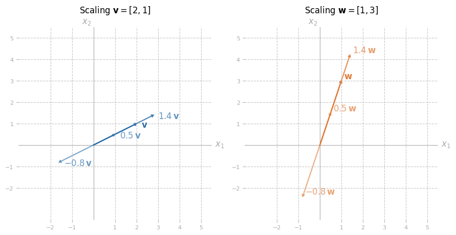
In general, multiplying a vector by a scalar scales the vector by the value of the scalar. Multiplying by 2 doubles the length of the vector. Multiplying by -1 reflects the vectors through the origin. It produces a vector pointing in the opposite direction.

Here are examples for the vectors $v$ and $w$ shown in the previous figures:

Linear Combination¶

Note, the usual order of operations applies. Multiply by the scalars before adding the vectors.

For example:

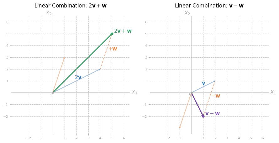
Here are two linear combinations of the vectors $v$ and $w$ illustrated earlier:

Vector Geometry¶

Since vectors may be represented with arrows, every vector has a length (magnitude) and direction.

Length/Magnitude¶

The length of a vector is found using the Pythagorean theorem. We denote the length of the vector $v$ with $\|v\|$.

In two dimensions:

For example:

The same formula generalizes to higher dimensions.

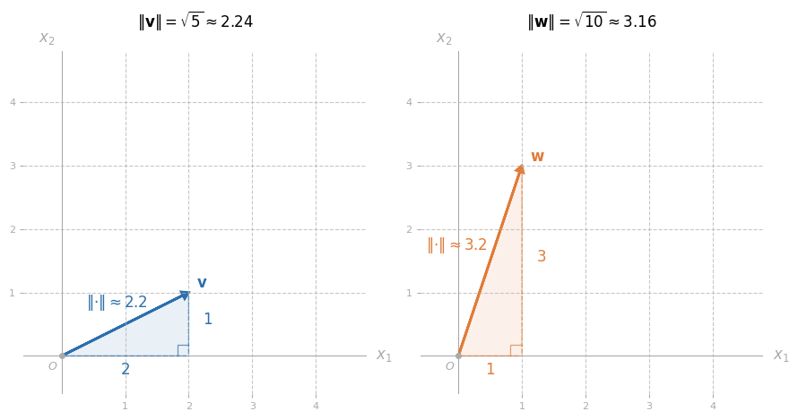
In other words, the magnitude of a vector is the square root, of the sum, of its entries squared. To find its magnitude, square every entry, add the squares, and square root the result.

For example, the magnitude of the vector $[3,4]$ is $\sqrt{3^2 + 4^2} = \sqrt{9 + 16} = \sqrt{25} = 5$.

The only vector of length zero is the zero vector: $[0,0,0...0]$. A vector is nonzero if at least one of its entries is nonzero.

Direction¶

The direction of a vector may be expressed by standardizing its length. To standarize, we normalize vectors:

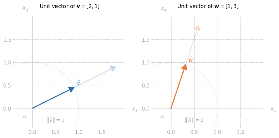
By normalizing, we produce a unit vector parallel to our original vector. This unit vector is the same for all vectors parallel to the original vector, so represents the direction of the vector. The unit vector always has length 1, so is independent of the magnitude of the vector.

Here are the unit vectors for the example vectors $v$ and $w$ illustrated earlier:

Two vectors, $v$ and $w$, are parallel if and only their unit vectors are identical, or are negations of each other (e.g. $\hat{v} = -\hat{w}$). Two vectors, $v$ and $w$, point in the same direction if and only if they share the same unit vector, $\hat{v} = \hat{w}$.

Angles and Inner Products¶

We can measure the angle between two vectors using an inner product:

For example, $[3,4] \cdot [-1,2] = 3 \times (-1) + 4 \times 2 = -3 + 8 = 5$.

Inner products are sometimes called “dot” products for the $v \cdot w$ notation.

We care about inner products since they are also related to the lengths of the two vectors, and the angle between them.

In other words, the inner product between two vectors equals the product of their lengths with the cosine of the angle between the two vectors.

We can rearrange this formula to find the angle between two vectors using their inner product.

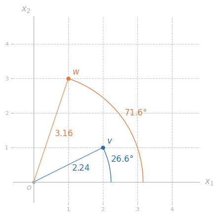
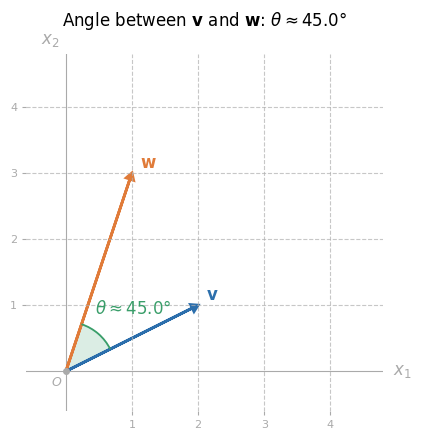
The two example vectors we’ve illustrated throughout are separated by about 45 degrees. You can check using their inner products and lengths.

We can use the inner product to test whether two vectors are perpendicular. The cosine of ±90 degrees is zero. The cosine of any other angle is nonzero. So, two vectors are perpendicular if and only if $\cos(\theta) = 0$. This requires $v \cdot w = 0$ since $\|v\| \neq 0$ and $\|w\| \neq 0$ when both are nonzero vectors.

For example, the vectors $[1,-1]$ and $[4,4]$ are perpendicular since $1 \times 4 + (-1) \times 4 = 4 - 4 = 0$. The vectors $[1,-1]$ and $[4,6]$ are not perpendicular since $1 \times 4 + (-1) \times 6 = 4 - 6 = -2 \neq 0$.

Exchanging Polar and Cartesian Coordinates¶

Polar to Cartesian¶

Suppose that $x$ is a point in a plane with radius $r$ and angle $\theta$ counterclockwise from the positive horizontal axis. Then:

Cartesian to Polar¶

Suppose that $x$ is a point in a plane with coordinates $x_1$ and $x_2$. Then:

The equation for $\theta$ is justified since: