Discrete Models - Data 89 Course Notes

This section will explore three famous discrete models. All of the models study random counts. These are random variables that take on integer values.

We will rely on a live code demo built into the textbook. To run the code, follow the instructions below.

Bernoulli¶

The simplest example of a random variable is a random variable that can only take on one of two values. When those values are 0 and 1, we call the random variable a Bernoulli random variable.

Since $X$ can either equal 1, or equal 0, we can specify the PMF of $X$ using only the chance that $X = 1$ , $\text{Pr}(X = 1) = p$ . The value $p$ is the success probability. By the complement rule, the chance $X = 0$ is, $\text{Pr}(X = 0) = 1 - p$ . The value $q = 1 - p$ is the failure probability.

The sentence: the random variable $X$ drawn from a Bernoulli distribution with success probability $p$ is usually expressed:

X \sim \text{Bern}(p)

(1)

where $\sim$ is the symbol for “drawn from”.

Notice that:

Every Bernoulli random variable is drawn from a categorical distribution on two categories, labelled “0” and “1”. Since the labels are arbitrary, Bernoulli random variables are often used to study settings where we are interested in a binary event. For example:
- Flip a coin. Label heads 1 and tails 0.
- Run an experiment. Label a succesful outcome 1 and a failure 0.
- Check a statement. Label a valid check 1 and an erroneous check 0.
Bernoulli random variables are often constructed from indicators. An indicator function for an event $E$ , is the function that returns 1 if $E$ happens, and 0 otherwise. We’ll see that many count variables can be expanded as combinations of indicators, where each indicator indicates whether or not some event occurs.
Bernoulli random variables are specified by the choice of the parameter $p$ . If we plot the PMF, then $p$ is the height of the bar assigned to the outcome $X = 1$ .
- The parameter $p$ is often called a success probability since we often use Bernoulli random variables as indicators for events we consider successes. For instance, if I am interested in whether a string of coin tosses contains at least 5 heads, I could define an event $E$ , which contains all strings with at least five heads and set $X$ to an indicator for the event. Then, when the event occurs (a success), my indicator equals 1. So, the chance of success is $\text{Pr}(X = 1)$ .
- If a Bernoulli random variable is constructed as an indicator for the event $E$ , then the success probability is the chance of the associated event, $p = \text{Pr}(E)$ .
- This language is arbitrary since the encoding to 0 and 1 is arbitrary. We could just as well call 0 success and 1 failure, but the assignment of 1 to success is so standard we will accept it as convention.

Experiment with the code cell below to visualize Bernoulli distributions:

from utils_dist import run_distribution_explorer

run_distribution_explorer("Bernoulli");

While simple, Bernoulli random variables:

Illustrate the two general approaches to defining a distribution. Either:
- Write down a process that produces the variable (e.g. I am interested in some event, and assign it an indicator $X$ )
- Or, fix the support and distribution function for the random variable.
Many random variables are specified by fixing a free parameter. The Bernoulli has only one free parameter, the success probability $p$ . Usually the parameters are either variables that can be toggled to change the shape of the distribution, so that it can be adapted to model the scenario of interest, or, are free variables involved in the definition of the process that produces the variable (e.g. the probability of the event that $X$ indicates).
Are a useful building block for other discrete disctributions.

Let’s build some other discrete distributions.

Geometric Random Variables¶

Suppose that you start flipping a coin. You are waiting to see a heads. Let $W$ denote the number of flips up to and including the flip when you see your first head. How is $W$ distributed?

As always, start with the support. The random variable $W$ is a count, so it must be integer valued. In order to see a head, we must flip at least once, so $W \geq 1$ .

Must $W$ be smaller than any upper bound $w \geq 0$ ? For instance, must $W \leq 10$ ?

No. While unlikely, it is possible to see ten tails in ten tosses. So, $W$ could be greater than 10. What about 20? The same logic applies. 50? The same logic applies.

No matter what $w$ you pick, it is possible, if very improbable, that $W > w$ .

This means that $W$ is unbounded above. In other words, the random variable $W$ is supported on the set of all positive integers $\{1,2,3,...\}$ . This is our first example of a random variable that can take on infinitely many values.

The fact that $W$ can take on infinitely many different values may be disturbing. So far all of our outcome spaces have contained finitely many outcomes. Do not fear. There is no issue extending to infinitely many outcomes. We just have to obey the axioms. In particular, we need to make sure our chance model, or PMF, assigns chances such that:

\sum_{w = 1}^{\infty} \text{PMF}(w) = \text{Pr}(W = 1) + \text{Pr}(W = 2) + \text{Pr}(W = 3) + \text{Pr}(W = 4) + ... = 1.

(2)

If the sum equals 1, then the distribution is normalized, so is valid.

A Note on Infinities

Not all infinities are alike. Some infinities are larger than others.

The set of all nonnegative integers is a countable infinity (or, countably infinite) since we can enumerate all the integers, place them in a list, and, if we started counting, we would reach any integer after a finite number of elements in the list. Just count in order:

0 \rightarrow 1 \rightarrow 2 \rightarrow 3 \rightarrow ...

(3)

After $n$ steps you will reach the integer $n$ , so every integer, $m$ will be reached in $m < \infty$ steps.

The set of all integers is also countably infinite. Count:

0 \rightarrow 1 \rightarrow -1 \rightarrow 2 \rightarrow -2 \rightarrow 3 \rightarrow -3...

(4)

You should convince yourself that this scheme will reach any integer eventually.

A rational number is any number that can be expressed as a ratio of all integers. It seems like the set of rational numbers should be much larger than the set of all integers since there are infinitely many rational numbers between every pair of integers. It turns out that the rationals are also countable, since there exists a scheme for listing every rational number in order, starting from 0!

In contrast, the set of real numbers (any number you can write as a decimal) is not countably infinite. It is uncountably infinite. There is no way to list all of the real numbers in order. We will see that, while there are no definitional problems writing down distributions for random variables with countably infinite support, uncountable infinities pose a subtler problem.

Now that we’ve established the support for $W$ , we should find one of its distribution functions. Since it is the most natural, let’s try and solve for its PMF.

To find the PMF, ask the question, what is the chance that $W = w$ ?

In order for the event $W = w$ to occur, we must fail on the first $w - 1$ tosses, and succeed on toss $w$ . So, we express the event $W = w$ as an intersection of $w$ events:

\{W = w\} = \{\text{fail on toss 1}\} \cap \{\text{fail on toss 2}\} \cap ... \{\text{fail on toss } w - 1\} \cap \{\text{succeed on toss } w\}

(5)

Since you are flipping a coin, the outcome of any toss is independent of the outcome of any other toss. Therefore, we can compute the chance of this joint event using the multiplication rule:

\text{Pr}(W = w) = \text{Pr}(\text{fail on toss 1}) \times \text{Pr}(\text{fail on toss 2}) \times ... \text{Pr}(\text{fail on toss } w - 1) \times \text{Pr}(\text{succeed on toss } w)

(6)

Notice, each toss is a binary event. It has two possible outcomes: heads (success), or tails (failure). So, we can represent each toss with a Bernoulli random variable. The Bernoulli has som success probability $p$ and failure probbility $q = 1 - p$ .

Since I am tossing the same coin repeatedly, the chance I fail or succeed on any particular toss is the same as any other toss. Therefore:

\text{Pr}(W = w) = q \times q \times ... \times q \times p = q^{w-1} p = (1 - p)^{w-1} p

(7)

You can read the equation above as, the chance I fail $w-1$ times ( $q^{w-1}$ ) times the chance I succeed on the last trial ( $p$ ).

Visualization Via an Outcome Tree

We can visualize the calculation described above using an outcome tree. Check the outcome tree below

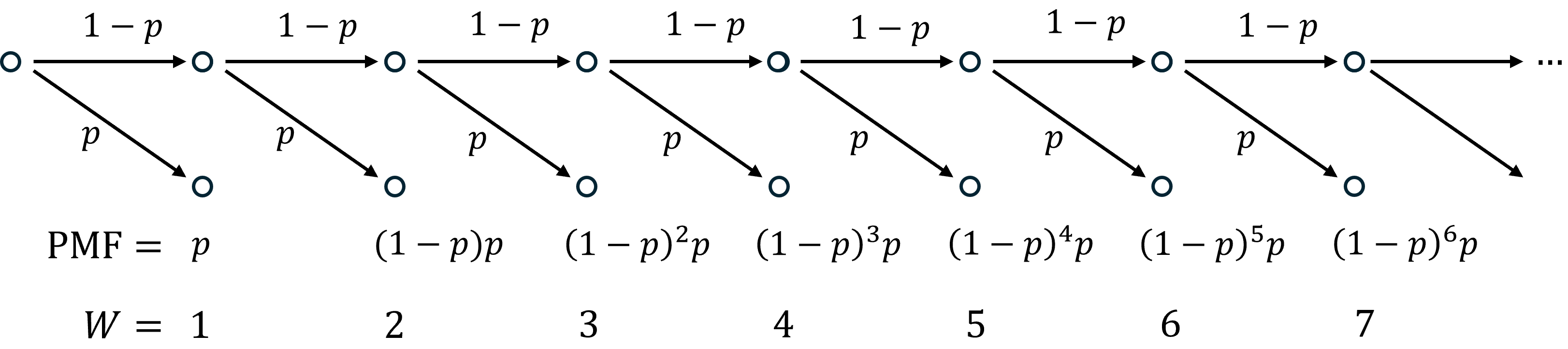
Horizontal arrows correspond to failed trials, diagonal arrows are successful trials. To find the chance of first succeeding in trial $W = 5$ , trace the path through the tree that ends at 5, then take the product of the chances for each arrow (each step in the process).

For a fair coin, $q = p = 1/2$ , so:

\text{Pr}(W = w) = (1 - p)^{w-1} p = \left(\frac{1}{2}\right)^w

(8)

We’ve plotted the PMF below:

Notice that, each bar is $1/2$ the height of the preceeding bar, since, on each toss, there is a $1/2$ chance of success.

Solution

The CDF starts at $1/2$ , since the chance of succeeding in 1 or fewer tosses is the chance of succeeding on the first toss, and increases with each subsequent toss since, the chance of succeeding at least once in $w$ tosses grows as we allow more tosses. The CDF approaches 1 since, the chance of no successes in $w$ tosses approaches zero for large $w$ .

The random variable $W$ is an example of a geometric random variable:

We denote the sentence, the random variable $W$ is drawn from a geometric distribution with parameter $p$ with:

W \sim \text{Geom}(p)

(10)

Like Bernoulli random variables, Geometric random variables have one free parameter $p$ which must be between 0 and 1.

The definition provided above is explicit. It defines the family of random variables by fixing a support (range of possible values), and form for the PMF.

We can also define geoemtric random variables implicitly, by identifying the types of processes that produce geometric random variables:

In other words, geometric random variables describe the number of attempts needed until a first success in a sequence of independent, identical, binary experiments.

Example

You roll a die repeatedly until you see a 4 or 6. Let $R$ be the number of rolls up to, and including, the first roll when you see a 4 or a 6. How is $R$ distributed?

First, recognize the process. $R$ is a random count, counting the number of trials in a sequence of independent and identical experiments. These experiments have only two outcomes. The roll is a four or a size, or the roll is neither a 4 nor a 6. Therefore, each experiment has binary outcomes, that can be encoded as indicators, so are equivalent to Bernoulli trials. It follows that $R$ must be a geometric random variable.

Geometric random variables are specified by a success probability, $p$ . The success probability $p$ is the chance any particular trial succeeds. To find $p$ , we need the probability that a die lands on a 4 or a 6. If the die is fair, then this chance is $2/6 = 1/3$ . Therefore:

R \sim \text{Geom}(1/3).

(11)

Therefore, the random variable $R$ has PMF:

\text{PMF}(r) = \text{Pr}(R = r) = \left(1 - \frac{1}{3} \right)^{r-1} \times \frac{1}{3} = \left( \frac{2}{3} \right)^{r-1} \frac{1}{3} .

(12)

Experiment with the code cell below to visualize Geometric distributions. Select “Discrete” then “Geometric” from the drop down. Adjust the parameter $p$ until you are confident you could explain how the shape of the PMF depends on $p$ . Try to explain, by interpreting $p$ as the chance of success in a string of independent, identical trials, why the shape depends on $p$ in the way you observed.

from utils_dist import run_distribution_explorer

run_distribution_explorer("Geometric");

Binomial Random Variables¶

Let’s construct a random count in a different way.

Suppose you flip a coin 10 times. What is the chance that, in 10 tosses, you see 7 heads?

Let $X$ denote the number of heads. As always, you should start by asking, *what is the range of possible values of $X$ ?

$X$ is a count so it must be integer-valued.
At least, all of the tosses are tails, so $X$ could be as small as 0.
At most, all of the tosses are heads, so $X$ could be as large as 10.

Therefore, $X \in \{0,1,2,3,...,10\}$ . In other words, $X$ is supported on all whole numbers between 0 and 10.

Next, let’s derive the PMF. To find the PMF, first ask a question of the kind, what is $\text{Pr}(X = x)$ ? Picka value $x$ that is in the support. Solve for the chance, then substitute for generic $x$ . For example, what’s the chance that $X = 7$ ?

The event $X = 7$ can happen in a few different ways. As usual, we’ll start by partitioning into all the ways the event can occur.

Here’s one $HHHHHHHTTT$ . Here’s another $TTTHHHHHHH$ . And here’s a third $THHHTTHHHH$ . All of these strings of tosses contain 7 heads and 3 tails.

What’s the chance we see the string $HHHHHHHTTT$ ?

This string is a sequence of events, so its a series of and statements. The outcome of your 5th toss has nothing to do with the outcome of your 7th toss, so the tosses are independent. Therefore, we can use the multiplication rule for independent events to split up each chance:

\begin{aligned} \text{Pr}(HHHHHHHTTT) & = \text{Pr}(H \text{ and } H \text{ and } ... H \text{ and } T \text{ and } T \text{ and } T) \\ & = \text{Pr}(H) \times \text{Pr}(H) \times ... \text{Pr}(H) \times \text{Pr}(T) \times \text{Pr}(T) \times \text{Pr}(T) \end{aligned}

(13)

We could, at this point, plu in $1/2$ for all the chances, but it will be more informative to keep the chance of heads and tails separate. So, let’s use $p$ for the chance of a heads (success) and $q = 1 - p$ for the chance of a tails (failure). Then:

\text{Pr}(HHHHHHHTTT) = p \times p \times ... \times p \times q \times q \times q = p^7 q^3.

(14)

This equation is suggestive. Notice:

The answer on the right hand side does not depend on the order of the heads and tails in the string defining the event, only the number of heads and tails. This is sensible. If we run a string of independent, identical experiments, then the chance of any sequence of outcomes should only depend on the number of times we saw each outcome, not their order. So, we can leave the right hand side alone, and replace the string $HHHHHHHTTT$ with any string of 10 characters, 7 of which are heads, and 3 of which are tails. We’ll need to count how many different strings satisfy this rule in a moment.
Each term has a clear source in the original question. We’ve raised $p$ to the 7th power since we asked about the chance of 7 heads. Since we are counting the number of heads with $X$ , the chance $X = 7$ is the chance $X$ takes on a particular selection drawn from its possible values, $x$ . So, anytime we ask a question, what is the chance we see $X = x$ heads, we should expect to see $p$ raised to the $x$ .
We’ve raised $q$ to the third power since, to see 7 heads in 10 tosses, we must see 3 tails. If we’d asked, what is the chance we see $X = x$ heads, we are equivalently asking, *what’s the chance we see $n - x$ tails $where$ n = 10$ was the number of tosses. So, we can rewrite the right hand side of the equation:

p^{x}q^{n-x} = p^x (1 - p)^{n-x}.

(15)

What we’ve just done is solved a specific case, then generalized the result to work for variants of our original question. Notice that, if we weren’t tossing a fair coin, but repeating some other binary experiment, then we could choose any success probability $p \in [0,1]$ .

Now, we’ve solved for the chance of seeing any specific string of $x$ successes and $n - x$ failures in a sequence of independent, identical, Bernoulli trials, each which succeeds with chance $p$ . We can put these together with the addition rule (marginalize) to recover the probability of seeing $x$ sucesses and $n - x$ falures:

\text{Pr}(x \text{ successes and } n - x \text{ failures}) = \sum_{...} p^x (1 - p)^{n-x}

(16)

where the ... stands for summing over all sequences of length $n$ , containing $x$ successes and $n - x$ failures. We’ve left this as a ... for now since it is too long for a subscript, and, since the next step won’t depend on the details of ...

Take a look at the sum again. The term inside the sum does not depend on the sequence chosen. So, it can be taken outside. Then the sum can be written:

\text{Pr}(x \text{ successes and } n - x \text{ failures}) = \left(\sum_{...} 1 \right) p^x (1 - p)^{n-x}

(17)

The sum of any constant $m$ times is $m \times \text{the constant}$ . The sum of the number 1 $m$ times is just $m$ . Therefore:

\text{Pr}(x \text{ successes and } n - x \text{ failures}) = |\text{all distinct sequences of }x \text{ successes and } n - x \text{ failures}| \times p^x (1 - p)^{n - x}.

(18)

In other words, the chance of $x$ successes in $n$ independent, identical, binary trials, is the number of ways of ordering $x$ successes and $n - x$ failures, times the chance of any particular sequence of $x$ successes and $n - x$ failures.

All that is left to do is to count the number of distinct ways we can arrange $x$ successes and $n - x$ failures.

Solution

\begin{aligned} \{& HHHHTT, \\ & HHHTHT,HHHTTH, \\ & HHTHHT,HHTHTH,HHTTHH,\\ & HTHHHT,HTHHTH,HTHTHH,HTTHHH,\\ & THHHHT,THHHTH,THHTHH,THTHHH,TTHHHH\} \end{aligned}

(19)

So, there are 15 distinct ways to arrange 4 heads and 2 tails.

Clearly, listing all the arrangements is too cumbersome for a long string. Even listing all the arrangements of 7 heads in 10 tosses would require listing 120 different arrangemenets.

So, we use combinatorics instead. If you haven’t solved this type of problem before, or its been a while, check Appendix A.1.

There are $n!$ distinct arrangements of $n$ distinguishable outcomes. If the outcomes are divided into two sets of sizes $x$ and $n - x$ , then we’ve overcounted by the $x!$ ways of rearranging the elements of the first set amongst themselves, and the $(n - x)!$ ways of rearranging the elements of the second set. So, the correct count is:

\text{number of arrangements} = \frac{n!}{x!(n-x)!} = \left(\begin{array}{c} n \\ x \end{array} \right)

(20)

We call the expression above a binomial or choose coefficient. We read it $n$ choose $x$ . The binomial distribution get’s its name from this coefficient.

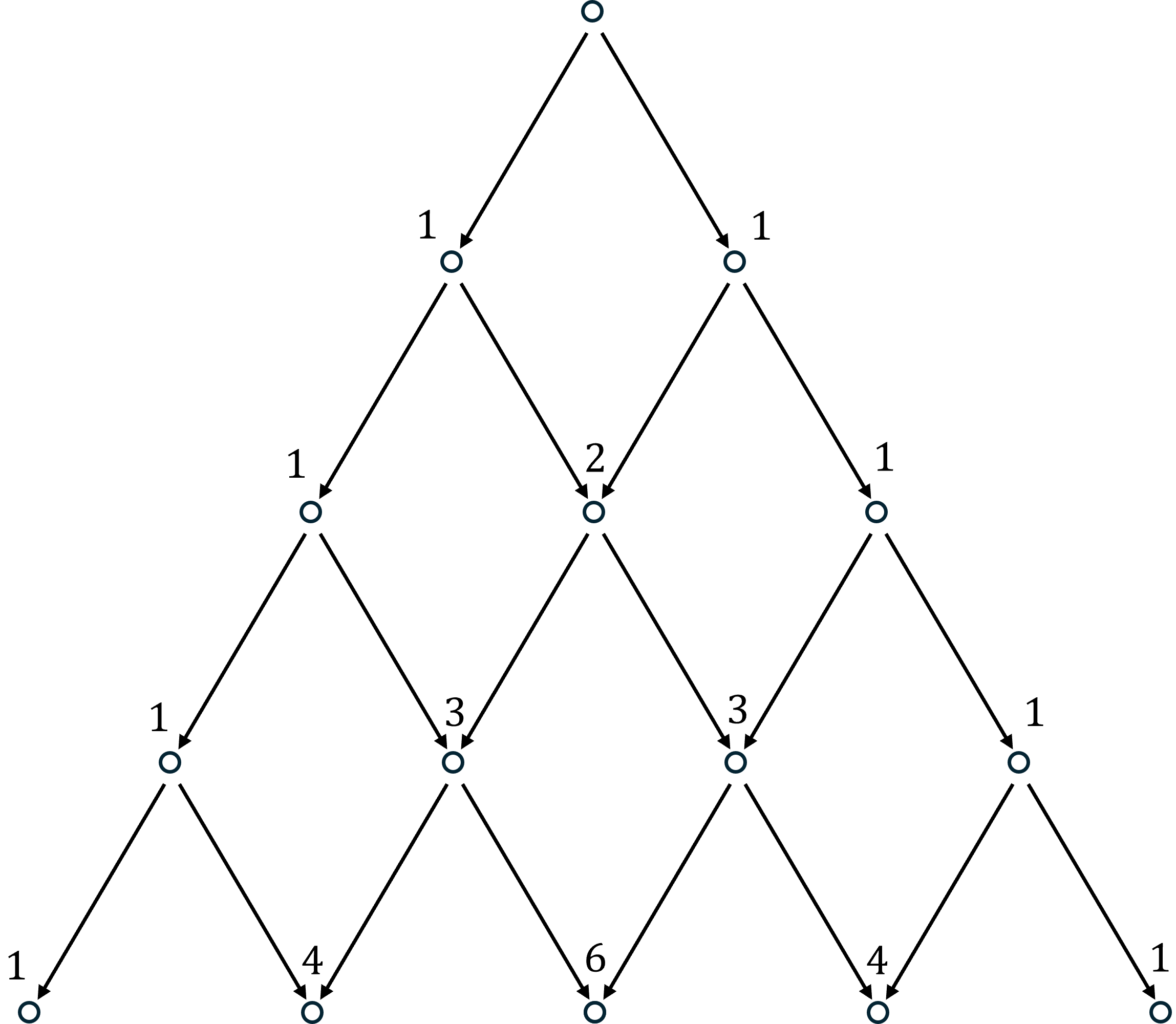
Visualization Via an Outcome Tree

We can visualize the calculation described above using an outcome tree. Check the outcome tree below for 4 trials, each which succeeds with chance $p$ :

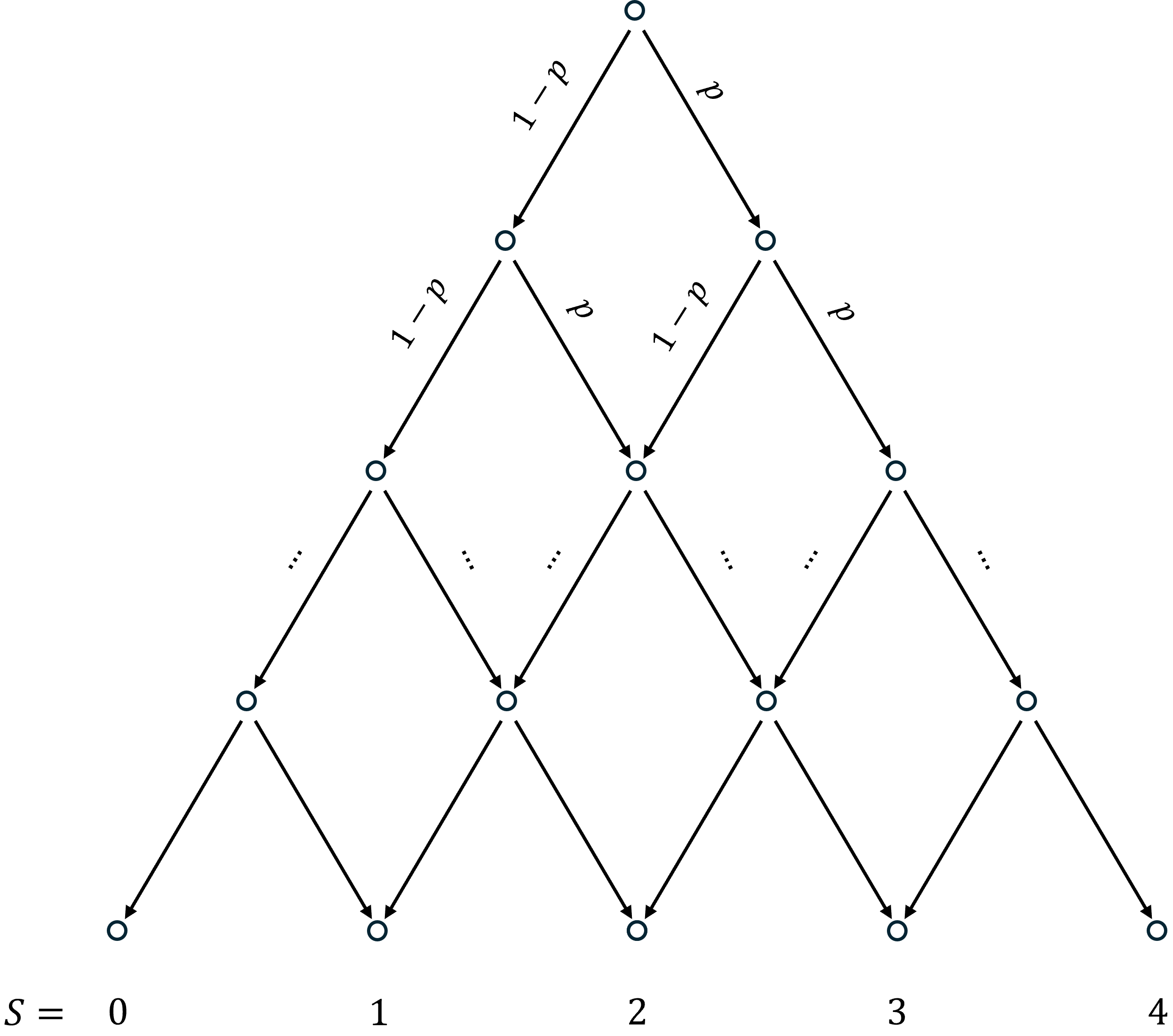
Diagonal arrows pointing left correspond to failed trials. Diagonal arrows to the right correspond to succesful trials. The vertical position of each node corresponds to the number of trials. The final horizontal position corresponds to the number of successes, $S$ .

Here’s an example sequence of trials that end with 2 successes:

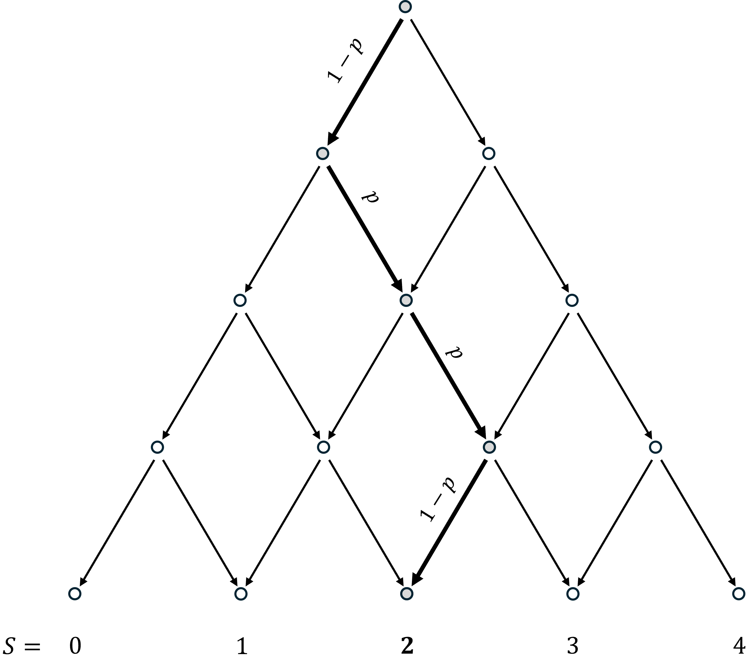
It corresponds to the sequence Fail, Success, Success, Fail. The corresponding chance is given by multiplying down the path. The chance is $(1- p) \times p \times p \times (1 - p) = p^2 (1 - p)^2$ .

Here’s a different sequence that also ends with 2 successes:

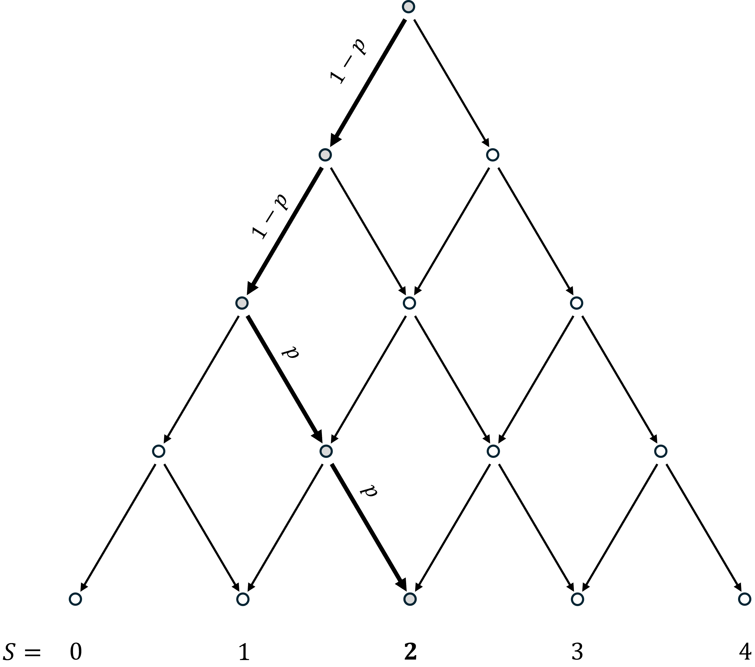
It corresponds to the sequence Fail, Fail, Success, Success. The corresponding chance is given by multiplying down the path. The chance is $(1- p) \times (1 - p) \times p \times p = p^2 (1 - p)^2$ .

The total number of paths pointing to 2 successes is $(4 \text{ choose } 2) = (4!)/(2!2!) = (4 \times 3 \times 2 \times 1)/(4) = 6$ (try drawing the other path). Therefore, the chance of 2 successes in 4 trials would be:

\text{Pr}(\text{2 successes in 4 trials}) = 6 p^2 (1 - p)^2

(21)

The outcome tree offers a nice alternative way to count the number of distinct sequences of $s$ successes in $n$ trials. Draw the tree again, pick a particular node in the tree, and look at all the arrows pointing into it. These represent all the numbers of successes you could have seen before the most recent trial. The most recent trial was always either a success or a failure, so if you are currently at $s$ successes, then in the previous round you were either at $s - 1$ or $s$ successes. In either case, the number of ways you could get to $s$ successes in $n$ rounds is the number of ways you could get to $s - 1$ in $n - 1$ plus the number of ways you could get to $s$ in $n - 1$ . So, we can count paths recursively. Start from the top of the diagram with a 1. Then, working down through the layers, set the number of paths into each node equal to the sum of the number of paths into all nodes that point to it. This builds Pascal’s famous triangle:

This is a nice way to count sequences when $n$ is small. When $n$ is large, use the choose formula.

Open up the drop down below to see all 6 paths that point to 2 success in 4 trials.

All Six Sequences

The six possible sequences with 2 successes and 2 failures is:

\{FFSS,FSFS,FSSF,SFFS,SFSF,SSFF\}

(22)

We now have all the pieces we needed to compute the desired chance. The chance of $x$ successes in $n$ identical, independent, binary trials is:

\text{Pr}(X = x) = \left(\begin{array}{c} n \\ x \end{array} \right) p^x (1- p)^{n-x}.

(23)

The random variable, $X$ , is an example of a binomial random variable. We can define it explicitly or implicitly.

We denote the statement $X$ is a binomial random variable on $n$ trials with success probability $p$ , with:

X \sim \text{Binom}(n,p).

(26)

Experiment with the code cell below to visualize Binomial distributions. Adjust the parameters $n$ and $p$ until you are confident you could explain how the shape of the PMF depends both. Try to explain, by interpreting $n$ and $p$ , why the shape depends on $p$ in the way you observed.

from utils_dist import run_distribution_explorer

run_distribution_explorer("Binomial");

Testing if a Die is Fair

In Section 1.2 we introduced a thought experiment. I offered you a six-sided die and claimed it was fair. You didn’t trust me, so you asked to test it out. You tossed it 10 times and saw the side labelled “4” 9 times. Suppose you saw the string:

4444446444

At the time we didn’t really have the tools to talk about how likely this outcome would be if the die was fair. Now we do.

The chance of seeing the exact string 4444446444 is the chance of seeing 4, then 4, then 4, then ... 6, then 4, ... then 4. This is a sequence of events, so is a string of “and” statements. To find its chance, use the multiplication rule. All the tosses are independent, so we can replace conditionals with marginals. This gives:

\begin{aligned} \text{Pr}(4444446444) & = \text{Pr}(4) \times \text{Pr}(4) \times ... \text{Pr}(6) \times ... \text{Pr}(4) \\ & = \text{Pr}(4)^9 \text{Pr}(6) & = \left( \frac{1}{6} \right)^9 \frac{1}{6} \\ & = \left(\frac{1}{6}\right)^{10} \approx 0.000000016 \end{aligned}

(27)

That’s about 16 in a billion, or one in a hundred million.

This seems like good reason to argue that the die is not fair. After all, we really shouldn’t see the same side so many times. But, you need to be careful here. This string is very unlikely, but it is just as unlikely as any other string of 10 outcomes. Look at the formula above. In the end, we just multiplied the chance of the outcome of each roll. Since we broke the probability into a product of probabilities that each roll returned some fixed value, we would get the same answer for any possible sequence, even sequences that look entirely plausible for fair die.

For example,

\text{Pr}(1456332114) = \text{Pr}(1) \times \text{Pr}(4) \times ... \text{Pr}(4) = \left(\frac{1}{6}\right)^{10} \approx 0.000000016.

(28)

Every specific string of 10 tosses is equally, and spectacularly, unlikely since they are all very detailed events. As usual, very detailed events have very small chances. In the end, all specific strings of lenth $n$ are equally likely, there are $6^n$ such sequences, so each has chance $(1/6)^n$ . Make $n$ big, and you can make each chance arbitrarily small.

This is a point worth remembering. In most situations, every detailed description of an outcome is both spectaularly unlikely, and an entirely normal coincidence, because all detailed events are coincidences.

If we can’t cast suspicion on the die by asking about the chance of the specific outcome, how can we show that the string 4444446444 really is suspicious?

Think again about what was suspicious in the original string. It wasn’t the order of the outcomes, nor was it the single “6” outcome. It was the sheer preponderance of “4”'s. The string is suspicious not because of all its detail, but because of a summary characteristic that is unusually unusual among all outcomes of ten die tosses. Just the statement, “of 10 tosses, 9 were on the same side” is suspicious by itself.

So, what’s the chance, if a die is fair, that in ten tosses, it lands on the same side 9 or more times?

Notice the structure of this question. We’ve asked for the chance that, if we tossed a fair die, we would see an event equally, or more suspicious, than the event we did observe, and we’ve been careful not to over-specify our event. By defining the event as generically as possible, we’ve made ensured that there are modifications of the event statement that could occur often. For example, the chance a fair die lands on the same side 2 or more times in ten tosses is quite large. It is the disparity in these chances that will allow us to build statistical evidence that my die was biased.

What’s the chance? Well, break down the event into each way it could occur:

We could see exactly 9 matched tosses, or exactly 10 matched tosses. Let’s call the number of matched tosses $X$ . Then we can write the probability of 9 matched tosses as the chance $X = 9$ , and the probability of 10 matched tosses $X = 10$ . These events are mutually exclusive, so their chances add.
We could see matches on any of the six sides. We weren’t really suspicious because it was the side labelled “4” that occured so frequently. We would have been equally suspicious had it been side “1” or side “6”. So, we can partition again by the side label that re-occurs. There are 6 options for the re-occuring side, and the events that the side “4” occurs $x > 5$ times and the side “2” occurs $x > 5$ are mutually exclusive. So, their probabilities add. Since all 6 are symmetric when the die is fair (we could relabel all the sides and would have no way to tell), adding their chances is the same as computing the chance for a specific side, then multiplying by 6.

So, let $X$ denote the number of times the side “4” appears in 10 tosses. Then the chance we are looking for is:

\begin{aligned} 6 \times \text{Pr}(X = 9) + 6 \times \text{Pr}(X = 10) = 6 \times (\text{Pr}(X = 9) + \text{Pr}(X = 10)) = 6 \times (\text{PMF}(9) + \text{PMF}(10)). \end{aligned}

(29)

To fill in the PMF’s, we need to recognize $X$ as a familiar random variable. The random variable $X$ is the number of times a die lands on the side “4” in 10 identical, independent tosses. If we call each toss an experiment, or trial, and consider each trial a success if we see a “4”, then $X$ is the number of successes in a sequence of 10 identical, independent binary trials. The success outcome is “rolled a 4.” The failure outcome is “did not roll a 4.”

This is exactly the implicit definition of a binomial random variable!

So:

X \sim \text{Bin}(10,1/6)

(30)

where the success probability parameter $p$ is $1/6$ since the chance we succeed in any trial is the chance any toss lands on a 6.

Then, we can just plug in the binomial PMF to find our chance:

\begin{aligned} \text{Pr}(\text{land on the same side 9 or more times in 10 tosses}) & = 6(\text{PMF}(9) + \text{PMF}(10)) \ & = 6 \times \left( \binom{10}{9} \left(\frac{1}{6} \right)^9 \left(\frac{5}{6}\right) + \binom{10}{10} \left(\frac{1}{6} \right)^{10}\right) \end{aligned}

Then, simplifying:

\begin{aligned} \text{Pr}(\text{land on the same side 9 or more times in 10 tosses}) & = \left( 10 \times \left(\frac{1}{6} \right)^8 \frac{5}{6} + 1 \times \left(\frac{1}{6} \right)^{9}\right) \\ & = \frac{50 + 1}{6^9} = \frac{51}{1,0077,696} \\& \approx 0.000005 \end{aligned}

(31)

That’s about 5 in a million. This time, we can draw a conclusion from this chance becuase there are similar event statements that are much more likely when the die is fair.

This is strong statistical evidence that the die is not fair.

Other distributions:¶

There are many discrete distribution models, each associated with a different family of distribution functions, and a different collection of generating processes. We’ve built a demo that you can use to explore some of the most important discrete distributions. You won’t need to know these all in detail, but this demo might be useful for you in future classes. We will ask you to interact with it on your HW.

If you’re interested in any of the other distributions, come ask the Professor. Given time, we’ll tough briefly on the Poisson.

from utils_dist import run_distribution_explorer

run_distribution_explorer();

Some General Lessons¶

Here are some last thoughts:

It’s worth remembering that there are two ways of defining a random variable, and associated distribution.
- The implicit approach is the most natural from an applied perspective. We’re interested in some random process in the world, have a natural language description of the process, and want to derive, from that description, the chances of events. Most of the important discrete distributions are tied to a particular story (natural language description of process), family of related stories. This approach is less common for distributions associated with continuous variables.
- All distributions can also be defined explicitly. Just like we can define a set in natural language (implicitly), then convert to an explicit list of elements, we can also define a distribution explicitly, by listing all the possible values of the random variable, then writing down a function that computes the chance of each event. Usually these functions have free parameters that are:
  - allowed to vary so that the modeler has the freedom to express many different distributions with a single function, and
  - allowed to vary to represent natural variants in the story associated with the distribution. For example, the parameters $n$ and $p$ of the Binomial distribution are naturally associated with a number of trials, and a chance of success per trial.
So, one skill you should develop is the ability to go back and forth between a functional form, with free parameters, and the shape of a distribution. It is very important that you understand how a distribution changes when we change its parameters. Understanding the parameteric dependence of chance means that you understand how the free elements of a question (e.g. the number of trials), influence the answer to your question. We’ll practice this skill explicitly in the next chapter. The better you get at it, the faster you’ll be able to make sense of equations, see how your answers depend on the set up to a question, gut check whether your answers are sensible, and, if asked to develop a new model, to choose a family of functions.