6.1 Taylor Series

Section 5.3 introduced the idea of a series. A series is a sum of infinitely many ordered terms.

This section develops a general method for approximating functions using series. This method is widely used in mathematics and in science. It allows accurate approximation of arbitrary smooth functions with polynomials.

Polynomial Approximation¶

Suppose that $f(x)$ is a smooth function of $x$. We are asked to approximate $f(x)$ for some $x$. For example, we could be asked for $e^{0.1}$.

Often, we can’t find $f(x)$, but can evaluate $f$ at some nearby $x_*$. For instance, $e^0 = 1$. If $f$ is smooth, then we can use information about $f$ at $x_*$, to approximate $f(x)$ when $x$ is close to $x_*$.

The simplest approximation is $f(x) \approx f(x)$. We can do better if we use more information.

Suppose that we know $f(x_*)$ for some $x_*$, and we know the slope of $f(x)$ at $x_*$, $\frac{d}{dx} f(x)|_{x = x_*} = f'(x_*)$.

Consider the tangent line:

This tangent line provides a good approximation for $f(x)$ when $x$ is close to $x_*$ since, by the limiting definition of a derivative:

The sign $\simeq$ means approximately equal to, and equal to in a limit. In this case, the limit is $\Delta x = x - x_* \rightarrow 0$.

Therefore, for $x$ near $x_*$:

The function $\tilde{f}_1(x)$ is linear in $x$. It passes through $(x_*,f(x_*))$ with slope $f'(x_*)$. We’ve denoted it $\tilde{f}$ to emphasize that it approximates $f$, and added the subscript $_1$ to emphasize that the approximation is a first order polynomial in $x$ (that is, a line).

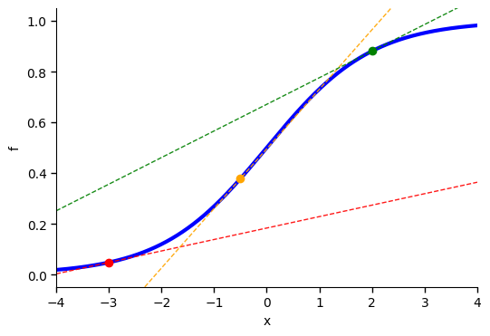
The figure below shows a smooth function $f$, and the linear approximations to $f$ at $x_* = -3$ (red), $x_* = -0.5$ (gold), and $x_* = 2$ (green). Notice that each linear approximation accounts for the slope of $f$.

We can develop higher order polynomial approximations by approximating $f'(x)$, then integrating. By the Fundamental Theorem of Calculus:

Then, for $y$ near $x_*$, use the linear approximation:

where the slope is now $f''(x_*)$ since $\frac{d}{dx} f'(x)|_{x = x_*} = f''(x_*)$.

Therefore:

Isolating $f(x)$ offers a quadratic approximation to $f$:

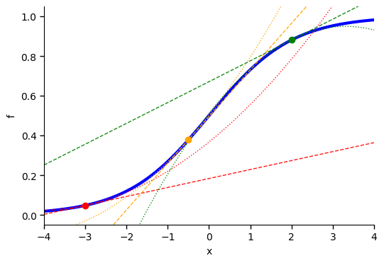
The figure below shows a smooth function $f$, and the linear (dashed) and quadratic (dotted) approximations to $f$ at $x_* = -3$ (red), $x_* = -0.5$ (gold), and $x_* = 2$ (green). Notice that each linear approximation accounts for the slope of $f$, while each quadratic approximation account for its slope and curvature at $x_*$. Also notice that the quadratic approximations are accurate farther from the points of expansion.

We can use quadratic approximations to help draw functions. If you are asked to draw $f$, and can evaluate both $f'$ and $f''$, then when you select reference points $x_*$ for plotting, check the slope and second derivative, then sketch the tangent, and the tangent parabola $\tilde{f}_2$.

Taylor Series¶

We can develop even better approximations by including more details about $f$ at $x_*$. If we account for $f'''$ then we can introduce a cubic approximation:

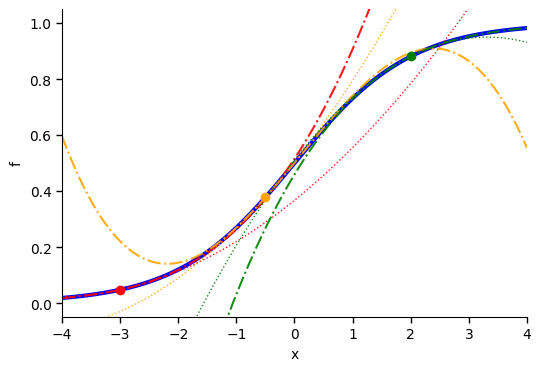
The figure below shows a smooth function $f$, its quadratic (dotted) and cubic (dash-dot) approximations at $x_* = -3$ (red), $x_* = -0.5$ (gold), and $x_* = 2$ (green). Notice that the cubic approximations are extremely accurate, even for $x$ far from $x_*$.

Taylor series generalize this idea by continuing the process out to infinitely many terms.

Quintic Approximation of the Logistic

The example function plotted in this chapter is the logistic function:

$$\text{logistic}(x) = \frac{1}{1 + e^{-x}}.$$

(28)

The logistic function is a popular function in statistics and machine learning, and is the heart of logistic regression. Let’s work out a fifth order approximation to the logistic function about $x_* = 0$.

The derivatives of the logistic function, evaluated at $x_* = 0$ are:

$f(0) = \text{logistic}(0)$	$f'(0)$	$f''(0)$	$f'''(0)$	$f^{(3)}(0)$	$f^{(4)}(0)$	$f^{(5)}(0)$
$\frac{1}{2}$	$\frac{1}{4}$	0	$-\frac{1}{8}$	0	$\frac{1}{4}$

All the even order derivatives except $f(0)$ equal zero since $\text{logistic}(x) - 1/2$ is odd about $x = 1/2$.

Therefore, the quintic approximation to the logistic is:

$$\text{logistic}(x) \approx \frac{1}{2} + \frac{1}{4} x - \frac{1}{48} x^3 + \frac{1}{480} x^5.$$

(29)

The approximation has errors that converge to zero at rate $\mathcal{O}(x^7)$ since $f^{(6)}(0) = 0$.

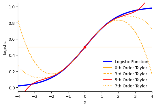
The quintic approximation about $x = 0$ is illustrated in red in the figure below. The seventh order approximation is illustrated as a dotted gold curve.

Notice that, adding the seventh order term only improves the approximation slightly. It is often true that we see diminishing returns as we add higher order terms to a polynomial approximation. This is especially true when we approximate bounded functions. It is also typical to see high order polynomial approximation swerve rapidly away from the function it is approximating after following it closely over some interval. Adding higher order terms generally widens the interval (though often with diminishing returns) while producing bigger errors outside the interval where the series is converging.

Examples¶

The two most important Taylor series in probability are the Taylor series of the exponential and the logarithm.

Exponential Functions¶

Suppose that $f(x) = e^x$. Then, let’s find its Taylor series about $x = 0$.

To find the Taylor series we need to work out all of the derivatives of $e^x$ at $x = 0$. This is easy, since the derivative of the exponential is the exponential:

Closing the recursion:

Therefore, $f^{(n)}(0) = e^0 = 1$.

It follows that:

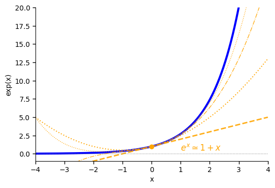
The figure below illustrates the first four approximations (linear, quadratic, cubic, quartic) to the exponential produced by its Taylor series about $x_* = 0$. In particular, $e^x \simeq 1 + x$. Higher order approximations are illustrated with lighter dotted curves.

To show that this series converges for all $x$, use the ratio test (see Section 5.3):

Since $r < 1$ for all $x$ the series converges for all $x$.

The Taylor series for the exponential gives us a new series that we can close. We can add it to the list we started with the geometric series:

The exponential’s Taylor series can be easily generalized to related functions via composition. For instance, if $f(x) = e^{g(x)}$, then:

Useful examples include:

1. $e^{\lambda x} = \sum_{n = 0}^{\infty} \frac{1}{n!} (\lambda x)^n$

2. $e^{-x} = \sum_{n = 0}^{\infty} \frac{1}{n!} (- x)^n$

3. $e^{-\frac{1}{2} x^2} = \sum_{n=0}^{\infty} \frac{1}{n!} \left( \frac{-1}{2} \right)^n x^{2n}$.

Truncating these series provides helpful approximations. For example:

when $x$ is small. This explains why, when we’ve drawn normal density functions (bell curves), we see a smooth parabola shape for $x$ near zero. That parabola is $1 - 0.5 x^2$.

Logarithms¶

The next most important example is the logarithm. We’ll Taylor expand the logarithm about $x_* = 1$ since the log diverges at $x = 0$.

To find the Taylor expansion, evaluate $\log(x)$, and its derivatives, at $x = 1$:

Closing the recursion:

for $n > 1$.

So, at $x_* = 1$:

Therefore:

Writing $x - 1 = \Delta x$ gives the concise form:

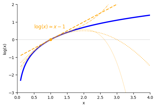
The figure below illustrates the first four approximations (linear, quadratic, cubic, quartic) to the logarithm produced by its Taylor series about $x_* = 1$. In particular, $\log(x) \simeq x - 1$. Higher order approximations are illustrated with lighter dotted curves.

To identify the region where the series converges, use the ratio test from Section 5.3:

The series converges if $r < 1$ and diverges if $r > 1$, so the Taylor series for the logarithm converges if and only if $|\Delta x| < 1$. This means that $\log(x)$ only equals its Taylor series about $x_* = 1$ for $x \in (0,2)$.

We can now add the log Taylor series to the list of infinite series we can close: