5.4 Categorizing Distributions by their Tails

In Section 5.2 we introduced methods that compare the rates at which different sequences converge. In Section 5.3 we showed that the rate at which a sequence converges determines whether or not sums of terms in the sequence (e.g. series) converge.

In this section we will apply the language developed in Section 5.2 to sort distributions by their tail decay rates. We will work from distributions that decay slowly to distributions that decay quickly. The integral convergence test established in Section 5.3 guarantees that the convergence arguments developed for series will extend to integrals.

Superexponential (Heavy) Tails¶

A distribution has heavy tails if it decays slowly.

In particular, a distribution has power law type tails if, for large $x$, it decays proportionally to $x^{-\gamma}$ for some $\gamma > 1$. We need $\gamma > 1$ when the random variable is unbounded, otherwise the distribution cannot be normalized.

Examples:

1. Discrete Power Laws:

   $X \in \{1,2,3,4,...,\infty\}$, $\text{PMF}(x) \propto x^{-\gamma}$ for $\gamma > 1$.

   Examples include word frequency in natural language, and degree distributions (number of connections) in random networks (e.g. social networks).

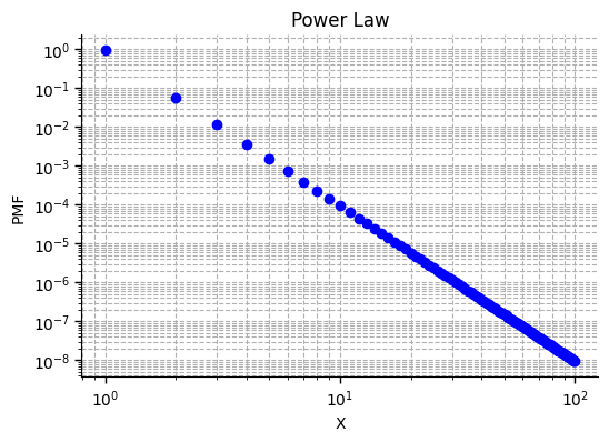
   Here’s an example with power $\gamma = 4$ on a log-log plot. Notice that, on the log-log plot, the power law is a straight line, and its slope equals the power, -4. Markers denote specific values of the PMF sequence $\{x^{-\gamma}\}_{x=1}^{\infty}$.

   

   You can experiment with discrete power law distributions using the Distribution Tail Explorer, or by running the code cell below. Try switching the $x$ and $y$ axes to log scales. You should see that, on a log-log scale, the bar plot follows a line, whose slope becomes more negative as you increase the power of the power law.

2. Pareto Distributions:

   $X \geq x_m$ for some $x_m > 0$, $\text{PDF}(X) \propto x^{-(\alpha + 1)}$ for some $\alpha > 0$.

   Examples include income and wealth distributions.

   Here’s an example with parameters $x_m = 1$, and $\alpha = 3$.

   

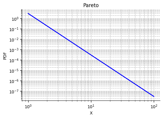
   Since $\alpha = 3$, the PDF decays according to a power law with power $\gamma = 4$. Notice that, on the log-log plot, the PDF is a straight line, and its slope equals the power, -4. Notice that the Pareto density and the power law PMF are identical functions, but the Pareto is interpreted as a density for a continuous variable so is evaluated on all $x \geq x_m.$

   You can experiment with Pareto distributions using the Distribution Tail Explorer or by running the code cell below. Try switchin to a log-log scale and varying the parameters.

3. Student’s t-Distributions:

   $$X \in (-\infty, \infty), \quad \text{PDF}(x) \propto g(x) = \left(1 + \frac{1}{\nu} x^2 \right)^{-\frac{\nu + 1}{2}}$$

   (1)

   for $\nu > 0$. In this case the tails decay proportionally to $x^{-(\nu + 1)}$ so $g(x) = \mathcal{O}(x^{-(\nu + 1)})$.

   Examples include estimated signal to noise ratios commonly used in hypothesis testing.

   Student’s t distributions are bell-shaped, but have slowly decaying tails. Here’s a log-log plot showing the student’s-t density as a function of $|x|$ with $\nu = 3$.

   

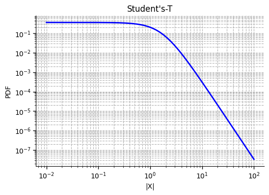
   The density is an even function, so it behaves symmetrically for negative $x$. When $\nu = 3$ the tails decay according to a power law with power 4, so on a log-log plot the density approaches a line with slope -4 when $x$ is large.

   You can experiment with $t$ distributions using the Distribution Tail Explorer or by running the code cell below. This time, just use a log plot for the $y$ axis since $\log(x)$ is undefined for negative $x$. Try increasing the free parameter $\nu$ that controls the shape of the distribution. Think about how $\nu$ controls the rate at which the tails decay. When $\nu$ is large, the log-plot will appear quadratic.

To detect power law tails, plot the log of the PMF (or PDF) against the log of $|x|$. If the resulting plot approaches a line for large $x$, then the distribution has power-law type tails.

Power law tails may converge slowly, especially when the power, $\gamma$ is close to 1. The smaller the power, the slower they converge. The larger the power, the faster the tails converge.

If $1 < \gamma \leq 2$ then the distribution exists but has infinite expected value. If $2 < \gamma \leq 3$ then the distribution exists and has a finite expected value, but has infinite variance and standard deviation. If $\gamma > 3$ then the distribution exists and has both finite expectation and finite variance.

Exponential Tails¶

A distribution has exponential tails if it decays at the same rate as an exponential function, $r^x$ for some $r \in (0,1)$. That is, if the tails are $\mathcal{O}(r^x)$ for some $r \in (0,1)$.

Examples:

1. Geometric Distributions:

   $X \in \{1,2,3,4,...,\infty\}$, $\text{PMF}(x) \propto (1 - p)^x$ for some $p \in (0,1)$.

   Here’s an example geometric distribution.

   

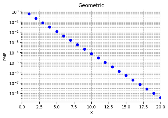
   We’ve used a log scale for the vertical axis (log of PMF) and a linear scale for the $x$ axis, so that the geometric sequence forms a line with slope equal to $\log(1 - p)$. Markers denote the sequence of PMF values for integer $x$.

   You can experiment with geometric distributions using the Distribution Tail Explorer or by running the code cell below. Try switching $y$ to a log scale. Leave $x$ on a linear scale. How does the rate of tail decay depend on the success probzability $p$?

1. Exponential Distributions:

   $X \in [0,\infty)$, $\text{PDF}(x) \propto e^{-\lambda x}$ for some $\lambda > 0$.

   Exponential distributions are often used to model continuous waiting times (see Section 6.2).

   Here’s an example exponential distribution.

   

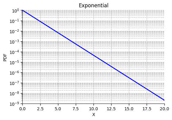
   We’ve used a log scale for the vertical axis (log of PMF) and a linear scale for the $x$ axis, so that the exponential PDF forms a line. Notice that, as the Pareto distribution is a to a discrete power law distribution, the exponential distribution is to the geometric distribution.

   You can experiment with exponential distributions using the Distribution Tail Explorer or by running the code cell below. Try switching $y$ to a log scale. Leave $x$ on a linear scale. How does the rate of tail decay depend on the parameter $\lambda$?

To detect exponential tails, plot the log of the PMF (or PDF) as a function of $x$ (not the log of $x$). If the log of the PMF (or PDF) approaches a line using a log scale on only the vertical axis, then the distribution has exponential tails.

Subexponential Tails¶

Examples:

1. Poisson Distributions:

   $$X \in \{0,1,2,...,\infty\}, \quad \text{PMF}(x) \propto \frac{\lambda^x}{x!}$$

   (2)

   for some $\lambda > 0$.

   Poisson distributions occur naturally in problems involving counts of rare phenomena, or of events that occur randomly in time.

   In this case the tails decay faster than exponential since $x!$ grows very quickly as a function of $x$. To a good approximation, $n! = \mathcal{O}(n^{n + 0.5})$ so $\lambda^x/(x!)$ converges to zero faster than $(\lambda/x)^x$. As $x$ increases, the fraction $\lambda/x$ decreases, so the base of the exponent is vanishing while the exponent is also diverging.

   You can experiment with Poisson distributions using the Distribution Plotter introduced in Section 2.5.

   Here’s an example Poisson PMF with parameter $\lambda = 8$ plotted using a log scale for the mass function and a linear scale for the input $x$. In this case the tail corresponds to large $x$.

   

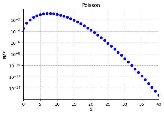
   Notice that, the log PMF is a concave function of $x$, so accelerates downwards as $x$ increases. As a result, the slope of the log PMF becomes more negative as $x$ increases, so the PMF converges faster than any exponential, which would form a line on the log PMF plot.

2. Normal (Gaussian) Distributions:

   $$X \in (-\infty, \infty), \quad \text{PDF}(x) \propto e^{-\frac{1}{2} x^2}$$

   (3)

   Normal, or Gaussian, distributions are the most widely used distributions in statistics. They define the classical bell-curve. They appear anytime we consider sample averages, or random numbers that are produced by sums of many independent and identical random variables. They are extremely common references for problems involving large sample sizes and estimates from large data sets. They are fundamental in the physical sciences, financial modeling, and a wide range of probability problems. Normal distributions have extremely light tails. They decay very quickly. The tails of the normal distribution are faster than exponential:

   $$\lim_{x \rightarrow \infty} \frac{e^{-\frac{1}{2} x^2}}{e^{-x}} = \lim_{x \rightarrow \infty} e^{-\left(\frac{1}{2} x^2 - x \right)} = 0$$

   (4)

   since $\frac{1}{2} x^2$ dominates $x$ for large $x$.

   You can detect Gaussian-type tails by plotting the log of the distribution against $x$. If the log of the distribution approaches a quadratic function for large $\pm x$, then the associated tail decays at a Gaussian rate, and is both subexponential (faster than exponential), and subpoisson (faster than Poisson).

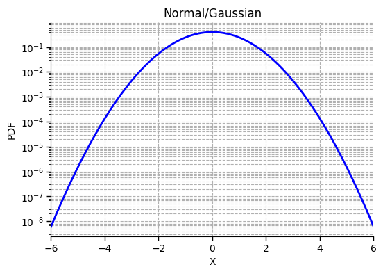
   Here’s a standard example. The log PDF, as a function of $x$, is simply the quadratic function $-\frac{1}{2} x^2$.

   

   You can experiment with Normal distributions using this Distribution Tail Explorer or by running the code cell below.