Function Operations - Data 89 Course Notes

A function operation is a procedure we can apply to transform or combine functions. Function operations are the essential tools that make mathematical modeling expressive. They are also the key to breaking complicated functions down into bite-sized pieces. The better you get at recognizing functions, and the richer your album of mental images, the more efficiently you will be able to break down formula into their pieces, visualize each piece, then visualize their combinations.

Linear Transformations...¶

to the Input: These transforms are used to generalize almost every distribution family. They need to be instinctive.
- Horizontal Translation: Replace $f(x)$ with $f(x - s)$ to translate the function horizontally by a shift $s$ . For example, $f(x - 3)$ looks like $f(x)$ shifted horizontally to the right by 3 units.
- Dilation: Replace $f(x)$ with $f(x/a)$ for some $a > 0$ to dilate the function. You can think of $a$ as controlling a zoom factor on the horizontal axis.
  - Using $a$ less than 1 compresses the function by making it narrower.
  - Using $a$ greater than 1 expands the function by making it wider. For example, setting $a = 3$ makes the function three times wider.
  - If $a < 0$ then the result also reflects $f$ about $x = 0$ .
- Generic: Replace $f(x)$ with $f((x - s)/a)$ .
to the Output: We can apply the same operations to the outputs of functions.
- Vertical Translation: Replace $f(x)$ with $f(x) + h$ to translate the function vertically by a height $h$ . For example, $f(x) + 2$ looks like $f(x)$ shifted vertically by 2 units.
- Vertical Scaling: Replace $f(x)$ with $c f(x)$ to scale the function. You can think of $c$ as controlling a zoom factor on the vertical axis.
  - Using $c < 1$ shrinks the function by making it shorter. For example, replacing $f(x)$ with $\frac{1}{3} f(x)$ compresses $f$ vertically by a factor of 3.
  - Using $c > 1$ expands the function by making it taller.
  - If $c < 0$ then the function reflects about the horizontal axis.
- Generic: Replace $f(x)$ with $c f(x) + h$ .

Maintaining Normalization

All distribution functions must be normalized. For instance, in Section 2.4 we saw that, for any PDF:

\int_{x = -\infty}^{\infty} \text{PDF}(x) dx = 1.

(1)

It is standard practice to define a generic family of models by setting $\text{PDF}(x) \propto g((x - s)/a)$ for some nonnegative function $g$ , shift $a$ , and horizontal dilation $a$ . These parameters are often called a location and a scale parameter. The location parameter controls the horizontal position of the distribution. The scale parameter controls its breadth.

The $\propto$ notation hides the normalization constant. This is useful, since the essence of a distribution is its shape, which is determined by the functional form $g$ . However, when $g$ depends on some free parameters, then we should always remember that:

\text{PDF}(x) = c(s,a) g((x - s)/a)

(2)

for some constant $c(s,a)$ that also depends on the parameters.

The location parameter has no effect on the normalizing constant since it just shifts the distribution. The scale parameter does. It can make the distribution wider or narrower. Just like a rectangle, if we make a distribution twice as wide, we double its area. So, to keep the distribution normalized, we must also always make it twice as short.

Generically:

\text{PDF}(x) = \frac{C}{|a|} g \left(\frac{(x - s)}{a} \right)

(3)

where $C$ is just a number determined by $g$ ( $C = 1/(\int_{x = -\infty}^{\infty} g(x) dx)$ ). That way, if we make the distribution wider by adjusting the scale parameter we also make it shorter.

Run the code cell below to visualize linear transformations of the inputs and outputs of a function. You’ve used this tool to check function properties. This time, experiment with the four sliders that perform horizontal translation, dilation, vertical translation, and scaling. Watch the grid lines in the background. These will translate, squash, and stretch, as you translate, dilate and scale. They represent the linear transformation of the original coordinate system.

from utils_week3_functions import show_function_properties
properties = show_function_properties()

Function Combinations:¶

Algebraic Combination:
- Function Addition and Multiplication: As they sound, $f(x) + g(x)$ or $f(x) \times g(x)$ .
  - Visualize the function sums like a stacked plot where the two functions sit on top of one another.
  - Visualizing function products takes practice, and is often best left to the tools from Sections 3.1 and Section 3.3. When given a product, always check the roots and sign of each term separately. Unfortunately, many distributions are expressed as products of functions.
- Linear Combination: This is a special version of function addition. It looks like $a f(x) + b g(x)$ for some coefficient $a$ and $b$ that scale each term in the combination.
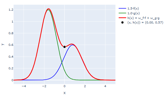
  - You can visualize a linear combination either by drawing its two component functions, $a f(x)$ and $b g(x)$ separately, then adding them together to produce the combo. The green and blue bumps are the component functions. The red curve is their linear combination. Varying $a$ or $b$ makes the associated bumps taller or shorter.
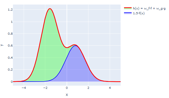
  - Alternately, you can use a stacked plot convention where you first draw $a f(x)$ , then you draw $a f(x) + b g(x)$ where the difference between your first curve and your second curve is $b g(x)$ . Here’s the same combination, using a stacked convention. In this example we drew the blue bump first, then added the green bump on top of it.
  - Important examples in probability are mixture distributions.
  Mixture Distributions
  To construct a mixture, sample in stages.
  For example, suppose that we have two large populations. We first pick a population to sample from at random, then, from that population, draw a sample of $n$ individuals. Then, we count the number of the sampled individuals who have a characteristic of interest and call our count $X$ . Suppose that, in the first population, 2 in 5 individuals have the characteristic, and in the second, 3 of 4 do.
  This process can be modelled as follows. First, draw a Bernoulli random variable $I \sim \text{Bernoulli}(p)$ where $p$ is the chance we select the second sample population. Then, if $I = 0$ , draw $X \sim \text{Binomial}(n,2/5)$ . If $I = 1$ , draw $X \sim \text{Binomial}(n,3/4)$ . Note, these shouldn’t be exactly Binomial since we usually sample without replacement, but, if the population is much larger than $n$ , its not a bad estimate.
  Then, what is the PMF for $X$ ? Well, we can find the chance that $X = x$ by partitioning, then using the multiplication rule. Alternately, draw an outcome tree. In either case:
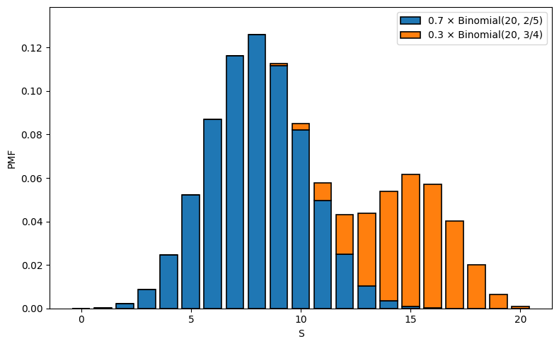
  $\begin{aligned} \text{PMF}(x) & = \text{Pr}(X = x) = (1 - p) \left(\begin{array}{c} n \\ x \end{array} \right) \left(\frac{1}{5} \right)^x \left(\frac{4}{5} \right)^{n - x}+ p \left(\begin{array}{c} n \\ x \end{array} \right) \left(\frac{2}{5} \right)^x \left(\frac{3}{4} \right)^{n - x} \\ & = (1 - p) \text{PMF}_{X|I = 0}(x) + p \text{PMF}_{X|I = 1}(x) \end{aligned}$
  (4)
  Here $\text{PMF}_{X|I = 0}(x)$ is the PMF when we draw from the first population, and $\text{PMF}_{X|I = 1}(x)$ is the PMF when we draw from the second. The resulting PMF is a mixture of the two PMF’s since it is a linear combination of the two.
  Here’s an example with $p = 0.3$ and with $n = 20$ . The colors represent the component distributions.

Run the code cell below to visualize function addition and multiplication.

from utils_week3_functions import show_function_combination
combination = show_function_combination()

Function Composition: The composition of $h$ and $g$ is $h \circ g(x) = h(g(x))$ . Many distributions are expressed as compositions.
- To visualize an arbitrary function composition, proceed as follows:
  Drawing composites
  1. Draw the inner function, $g(x)$ , and the outer function $h(x)$ . Clearly distinguish them with different colors or markers so you don’t mix them up.
  2. Add to your plot the line $y = x$ . This line is useful since we can use it to exchange inputs and outputs.
  3. Work an input at a time. Pick some $x$ . Add a point at $(x,0)$ on the x-axis. Trace a lightly dashed line vertically upwards so you can remember where you started.
    Next, add a point at $(x,g(x))$ where your dashed vertical meets $g(x)$ . We’ve now produced the output of the inner function.
    To pass the output of the inner function into the input of the outer function, trace horizontally across from $(x,g(x))$ to $(g(x),g(x))$ . This is the intercept between the horizontal line passing through $(x,g(x))$ and the $y = x$ line. Then, trace vertically from $(g(x),g(x))$ to $(g(x),h(g(x)))$ . This is the intercept of a vertical line leaving $(g(x),g(x))$ and intersecting the outer function $h$ .
    We’ve now recovered $h(g(x))$ . To plot it at the correct input, trace horizontally until you intercept the lightly dashed line leaving the original $x$ . That is, from $(g(x),h(g(x)))$ to $(x,h(g(x)))$ .
- This process is a bit involved at first, but it’s a nice visual procedure. Once you get the hang of it, you can use it to very quickly evaluate compositions of arbitrary $h$ and $g$ . Just repeat the process for a bunch of different $x$ values. It is good practice to try this by hand at least once.

Run the code cell below to visualize the composition of two functions.

from utils_week3_functions import show_function_composition
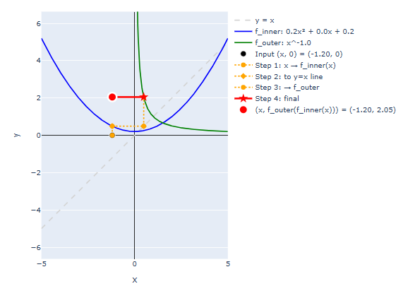
composition = show_function_composition()

The dashed orange lines represent the procedure provided above. Try building up an example composition. A good place to start is $f(x) = e^{-\frac{1}{2} x^2 + 1}$ where the inner function $g$ is a negated quadratic and the outer function is an exponential. You’ll practice with this example in discussion.

Here’s a different example with $f(x) = h(g(x))$ with $g(x) = 0.2 \times(1 + x^2)$ and $h(x) = 1/x$ .

Building Distributions as Composites

These are both examples where the inner function is convex or concave, and the outer function is both monotonic and nonnegative. This recipe inner concave, outer monotonically increasing and nonnegative is a good procedure for building density functions. The outer function ensures that the composition returns a nonnegative number. It is usually selected so that it converges to zero in a limit that can be achieved by the inner function.

We can also use three-dimensional plots to visualize function compositions. Set the first axis to the input, $x$ , the second to the inner function, $g(x)$ , and the third axis to the composition $h(g(x))$ . If we plot $g$ as a function of $x$ , and $h$ as a function of $g$ , then we can recover $h(g(x))$ as a function of $x$ .

As an example, run the code cell below. Set the inner function to $g(x) = \frac{1}{2} (x^2 + 1)$ . Set the outer function to $h(x) = 0.5^x$ .

Click “Show Inner” to show the quadratic function. Then click “Show Outer” to show the exponential function.

Then click “Compose” to reveal the composite (dark red). Move the cursor to vary the input $x$ .

from utils_week_4 import show_composite_3d
composition_3d = show_composite_3d()

Inverses:¶

If $f$ is monotonic, then it is invertible. Its inverse, $f^{-1}$ is the function that accepts outputs of $f$ and returns the matching input.

In other words, given $f(x) = y$ , $f^{-1}(y) = x$ .
It can help to think, whatever $f$ does, $f^{-1}$ undoes.
Inverse are constructed by reflecting $f$ about the $x = y$ line (exchange inputs and outputs).
- To reflect, do the following:
  Drawing Inverses
  1. Draw $f(x)$ .
  2. Draw the line $y = x$ which exchanges inputs and outputs.
  3. Sketch the reflection of $f$ across $y = x$ .
  4. If you struggle to sketch the reflection, work one input at a time:
    Select some $x$ . Add a point at $(x,f(x)).$
    Trace horizontally to $(f(x),f(x))$ . This is the intercept of the horizontal line through $(x,f(x))$ with the $y = x$ line.
    Trace vertically from $(x,f(x))$ to $(x,x)$ .
    You now have two sides, and three corners, of a square. Complete the square by adding in the missing corner at $(f(x),x)$ . You have now swapped the inputs and outputs of $f$ . This new point is the reflection.
  5. Repeat this process for many inputs. The resulting curve is the inverse function since it accepts outputs of $f$ , and returns the matching inputs.
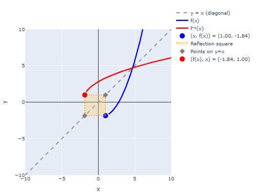
- The image below shows an example. The blue function if $f$ , the dashed grey line is the $y = x$ line that matches inputs and outputs, and the red curve is the inverse produced by reflecting across $y = x$ . The orange filled square is the square used to build the reflection.

The most important examples in probability are the exponential and logarithm functions. Remember $e^{\log(x)} = x$ and $\log(e^{x}) = x$ .

Run the code cell below to visualize function inverses. Start with a linear function, and see how the inverse varies as we vary the initial function. The square you see represents the graphical construction outlined above. It is good practice to try this by hand at least once.

from utils_week3_functions import show_function_inverse
inverse = show_function_inverse()

Once you’ve run the code below, go back to the composition demo provided above, and pick inner and outer functions that are related by an inverse. For example, $e^x$ and $\log(x)$ . Then, the graphical construction used to create the composite will trace the boundary of the reflecting square, always returning the $(x,x)$ corner. In other words, $f^{-1}(f(x)) = x$ .

Applications of Inverses in Probability

Why care about inverses?

Inverse functions are extremely useful in applied problems. Here are two:

Finding Thresholds for Statistical Tests: It is common practice to run a statistical test by collecting some data, using it to compute a test statistic (e.g. the sample mean), then to compare the observed value of the test statistic to a threshold. Since data is almost always random, the observed test statistic is random, so we’ll denote it $T$ . We’ll denote the threshold $t_*$ . Often we pick the test statistic so that its value measures how much the observed data disagrees with what we would expect, or is typical, under some hypothesis. Usually, the larger the test statistic, the more evidence we have that the hypothsis is false. Formally, we pose a chance model for $T$ that should hold under the hypothesis. Then, we select the threshold so that, if the hypothesis were true, then $\text{Pr}(T \leq t_*) = 1 - \alpha$ for some desired $\alpha$ close to zero. That way, if we observe $T > t_*$ , then the observed data would have been suspiciously atypical had our hypothesis been true. This is usually considered statistical evidence against the hypothesis. The chance, $\text{Pr}(T > t_*)$ is the (inf)famous “p”-value.

The level $\alpha$ controls how conservative, and how sensitive, our test is. You can think of it as the chance that the test falsely rejects if the hypothesis is ture. It is the level of evidence we demand in order to reject the hypothesis.

We usually start by fixing an $\alpha$ (e.g. $\alpha = 0.05$ or $\alpha = 0.01$ ), then solve for the associated threshold $t_*$ . Notice that, $\text{Pr}(T \leq t_*) = \text{CDF}(t_*)$ . Then, our original equation was:

\text{CDF}(t_*) = 1 - \alpha

(5)

so, to find the desired threshold, we should use:

t_* = \text{CDF}^{-1}(\alpha).

(6)

Sampling: Suppose that you wanted to draw a random variable $X$ with a specific CDF, $F_x$ . How would you do it?

Here’s an algorithm:

First sample a uniform random number $U \sim \text{Uniform}([0,1])$ . Most pseudorandom number generators due this by exploiting some of the properties of continuous random variables introduced in Section 2.3. Namely, if we draw some continuous random variable $Y$ , then, no matter its PDF, if we drop the first $d$ digits of $Y$ and multiply by $10^{(d - 1)}$ then we’ll get a random variable between 0 and 1 that is essentially uniform if $d$ is big enough. Continuous random variables look uniform on sufficiently small intervals. In practice, many computers look up the time when you trigger a computation, drop most of the leading digits, then use the remainder to make a uniform number.
Convert the uniform random variable into the desired random variable $X$ via $X = F_x^{-1}(U)$ .

Why does this work?

Well, let’s find the CDF of $X$ :

\text{CDF}(x) = \text{Pr}(X \leq x) = \text{Pr}(F_X^{-1}(U) \leq x).

(7)

All CDF’s are monotonically nondecreasing functions, so their inverses are also monotonic. Therefore: $F_X^{-1}(U) \leq x$ is the same statement as $U \leq F_X(x)$ . Therefore:

\text{CDF}(x) = \text{Pr}(F_X^{-1}(U) \leq x) = \text{Pr}(U \leq F_X(x)).

(8)

Then, since $U$ is uniform we can use probability by proportion:

\text{CDF}(x) = \text{Pr}(U \leq F_X(x)) = \frac{|F_X(x) - 0|}{|1 - 0|} = F_X(x).

(9)

Notice, this will work for both discrete and continuous variables since it is based on the CDF, which is defined in the same way for both. We need to be a little more careful with our inverse definition for the discrete case, but there are no issues if we restrict the outputs of the inverse to the support of the target variable. This is the standard sampling protocol used by most random number generators.

3.2 Function Operations

Linear Transformations...¶

Function Combinations:¶

Inverses:¶