In Section 2.3 we showed that, for any continuous random variable , the chance equals some exact value, , is zero, no matter which we choose. As a result, the PMF is zero everywhere:
This tells us nothing about the random variable except that it is continuous. It does not tell us how to compute chances.
In this chapter we will introduce our last type of distribution function, a probability density function. Density functions are the continuous analog to mass functions for discrete random variables. If you are asked to picture a distribution in your head, and you picture a bell-curve, or a bell-curve shaped histogram whose bars could be made very narrow, then you are picturing a density function.
This section will introduce density functions by experimentation with histograms for continuous random variables. Once we see that density is a natural idea for continuous random variables, we’ll show how to relate densities to chances, then introduce some examples.
Read Me to Run Live Code!
At the top right of your screen you should see a “power” button symbol. This is the “Live Code” button. It starts a Jupyter kernel. You will need to click it before running any demos.
Click it now. You should see a green progress bar spin about the button for a bit. When the button vanishes and is replaced with a menu of buttons (e.g. the play button) then your kernel has started and you can start running the demos.
When you see a code cell later, click the play button on the code cell to generate the interactive demo.
Probability Density
By Experiment
Let’s start with an experiment. We’ve already seen that we can:
Define uniform continuous variables by equating chances to proportions of length or area
Relate chances of events to long run frequencies
Define arbitrary continuous random variables by fixing a cumulative distribution function (CDF).
Let’s set up an experiment that puts these ideas to work. We’ll start with a uniform continuous random variable, transform it to get something non-uniform, divide up its support into small pieces, then draw many copies of the variable and see how frequently it lands in each piece. Since probabilities equal long run frequencies, the associated histogram will represent a distribution function. Formally, its a categorical distribution with categories equal to the histogram bins. The key continuous idea is, we have the freedom to change the width of the bins.
To get a detailed picture of the distribution, we’ll try to take a limit where the bins get arbitrarily small. Per Section 2.3, we’ll see that, making the bins narrower, lowers the frequency that outcomes land in each bin, so to keep the histogram bars about the same height as we narrow the bins we’ll have to scale by the width of the bins. Scaling by width produces a density. Once we’ve seen a density, we’ll show that, unlike the PMF, the density function can be used to recover a CDF. Then, since a CDF specifies a measure, the density function is enough to define a probability model.
Imagine you are throwing darts at a dartboard. We’ll imagine that you’re not very good at darts, so the position of each dart is uniform over the board. For a circular board this means we are picking a location uniformly from the interior of a circle.
This is a uniform continuous model, so we can measure chances. The chance a dart lands in some region on the board, is:
where is the collection of all possible positions the dart could land (the circular board).
You want your darts to land near the center of the board. So, you decide to measure the distance the dart lands from the center. The dart’s position is random, so is it’s distance from the middle of the board. We’ll call that random variable for radius.
is a continuous random variable. For simplicity, let’s assume the dart board has radius 1. Then, is supported on the interval since we, at best, hit the center of the board, and, at worst, hit the outer edge.
Is uniformly distributed? Take a moment to think about this carefully before answering.
If you’re unsure how to proceed, remember that its often easier to start with a CDF.
What is:
Well, the region on the board where is the interior of a circle centered at zero, with radius . We don’t have to worry about the distinction between and since the position of the dart is continuous. We can now visualize the event as a filled circle with radius inside a larger circle of radius 1. The chance we land in the inner circle is the ratio of its area to the area of the full circle.
So, using probability by proportion:
To check whether this CDF could correspond to a uniform measure, let’s compare the chances that lands in two intervals of equal length. For instance, what are the odds that compared to the odds ?
So, the dart is 3 times more likely to land in the outer interval, than the inner interval, . The dart’s distance from the origin cannot be uniformly distributed. It is more likely to land farther from the center of the board than closer to the center.
To visualize this bias, run the following experiment:
Throw a bunch of darts (sample uniformly from the circle),
Compute the distance of each dart from the center (sample repeatedly), then
Divide the interval into many small pieces, count the frequency with which lands in each segment, and
Plot the associated histogram.
We’ll let denote the width of the histogram bins. Remember, we get to choose these. They are an artifact of our visualization scheme. To get a precise picture, we will want to both take many samples to eliminate randomness in the bar heights and make the bins very narrow.
You can run this experiment yourself using the demo below:
from utils_dartboard import run_dartboard_explorer

run_dartboard_explorer(R=1.0)<utils_dartboard.DartboardVisualization at 0x20ed14ffd10>If you draw enough samples, and keep the bins small enough for a detailed plot, but big enough that they each contain a lot of samples, then you should get a pretty clear picture. The histogram should look something like this:
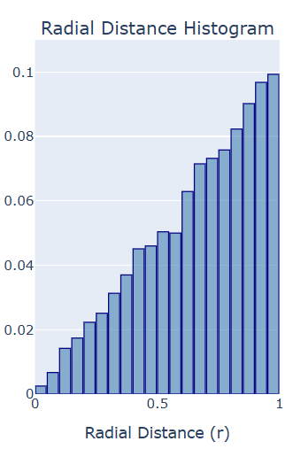
It’s basically a linear wedge. A linear trend is not surprising, since running sums act like integrals, the integral of a linear function is quadratic, and we saw that the CDF is a quadratic function of .
So, it’s natural to think that, the distribution of should be described by some linear function of . To recover that function, we need to make sure our histogram plot is not sensitive to arbitrary choices we made when we set up the experiment.
There were two free parameters in the set up:
The number of samples, and
The bin widths, .
To see why these are problematic, open the demo again, and set the vertical heights of the bars equal to the raw number of samples that land in each interval. This is the simplest histogram convention. The height of each bar is the number of times the corresponding event occured.
from utils_dartboard import run_dartboard_explorer

run_dartboard_explorer(R=1.0)<utils_dartboard.DartboardVisualization at 0x20ee89c6e90>Now try varying the number of samples. If you increase the number of samples to make the plot less noisy, you should see that all the bars get taller. The histogram is still roughly linear in but its slope changed.
The distribution of was fixed by the sampling process, so cannot depend on the total number of samples. Accordingly, we can’t equate probability to a raw count of occurences. That’s not surprising. Probabilities should match long run frequencies.
So, to make sure that our plot is invariant to (does not depend on) the total number of samples, we should set the height of the bars to the frequency with which each event occured. This converts to plotting chances rather than counts.
Set the y-axis back to frequency and try varying the sample size. You should see that, as long as you keep the bin widths fixed, the histogram now converges to a fixed function in the limit of many samples. This function is a categorical distribution on the bins. It is analogous to a PMF when we round to some fixed, finite, precision.
So far so good. Albeit, our plot could still depend on the bin widths.
Keep plotting frequency, and this time try varying the bin width.
from utils_dartboard import run_dartboard_explorer

run_dartboard_explorer(R=1.0)
You should see that, if you make the bins wider, not too much changes except the bars get taller, but, as you make the bins smaller, things start to fall apart. The narrower the bins, the shorter the bars, and the noiser the pattern. The second effect, the amount of noise, can be fixed by increasing the sample size.
So, take a very large sample size, and see how small you can set the bars. Can you set the bars small enough so that their height stops changing?
from utils_dartboard import run_dartboard_explorer

run_dartboard_explorer(R=1.0)
No!
Everytime you shrink the bins, the bars get shorter. The function we’re looking for is still linear, but its slope depends on the arbitrarily chosen bin width. Worse, its slope approaches zero as we make the bins narrow.
That last observation is the main result of Section 2.3. If a random variable is continuous, then the chance it lands in a shrinking series of intervals decreases as the intervals get narrower, and approaches zero as the intervals converge to a point. The distance from the center of the board, , is a continuous random variable, so the chance lands exactly in any very narrow bin must be very small. What we’re seeing is experimental evidence that, for a continuous random variable, the chance of every exact event is zero, so its PMF is zero everywhere.
Ok, what next?
Well since the heights of the bars decrease as we make the bars narrow we could try an old trick from calculus. Let’s scale the heights of the bars by dividing each frequency by the width of the associated bin. Then we’re plotting frequency per bin width. Hopefully, dividing by the shrinking bin width should cancel out the decrease in frequency.
Try it! Set the y-axis convention to frequency per width (density).
from utils_dartboard import run_dartboard_explorer

run_dartboard_explorer(R=1.0)<utils_dartboard.DartboardVisualization at 0x20ee8a84e90>Now you should see that, as long as you keep increasing the sample size, the histogram converges to the linear function: . This function stays stable no matter how you vary the bin widths, or the sample sizes, as long as we have enough samples to average away noise in the frequencies!
To check, lock the bin width, , to a function that decreases in sample size, , so that the bin widths approach zero as the sample size diverges, and do so slowly enough so that the number of samples in each bin increases as increases.
Click the “lock” checkbox, then gradually increase the sample size.
from utils_dartboard import run_dartboard_explorer

run_dartboard_explorer(R=1.0)
What we’ve just recovered is a probability density function. We call it a density by analogy to mass per volume.
In physics, the density of a region is the ratio of its mass to its volume. We can define the density of a point by using arbitrarily small regions. For instance, the density of a point is the total mass within of , divided by the volume of the region of points within of , in the limit as goes to zero. We call frequency per length a density since it has units of probability mass per length. This definition extends naturally to higher dimensions. We can define densities as probabilities per unit area or probabilities per unit volume.
Working with densities will help us resolve one of the paradoxes from the end of Section 2.3. There we saw that, when we sample a continuous random variable we always get a specific outcome despite the fact that every specific outcome has zero chance. Somehow, all of the possible outcomes had zero chance, but collections of outcomes had nonzero chances.
Density and mass behave the same way. The total mass in some region vanishes as we make the region arbitrarily small. So, the total mass at any point is zero. Yet, regions are composed of points, and can have nonzero mass.
This paradox is resolved by integration. The total mass of an object is not the sum of the masses of every infinitesimally small piece of the object. It is the integral of the density of every point in the object.
The same thing will be true for probability densities. Let’s check it for our example.
We’d proved that:
using probability by proportion.
Then, by experiment, we’d guessed a density function:
The region is the interval since is a radius. Therefore, we should try integrating the density from 0 to :
Therefore, in this example probability mass (e.g. chances) are related to densities by integration:
We’ll see that this is always true for densities, and that we can use this relation to define continuous random variables starting directly from density functions. This approach is more intuitive than starting from cumulative probabilities, since density functions look like histograms. CDF’s don’t.
Definition and Relation to Chance
Let’s formalize our construction.
It is very common to denote:
The PDF of a continuous random variable, , evaluated at : . Here we use a subscript to remind us which random variable, and a little for function.
The CDF of a continuous random variable, , evaluated at : . Here we use a subscript to remind us which random variable and use a capital for function.
We use a lower case for the density and an upper case for the CDF since this notation matches the standard convention in calculus. We’ll adopt this notation since it is so widely used, but frequently remind you that little is the PDF, while is the CDF.
The PDF and PMF are easy to mix up since the PDF looks like a rescaled limit of a PMF, when we make our intervals very narrow. This idea is more than an annoying stumbling block. The relationship between PDF, and its approximation with a PMF, explains how we should use PDF’s to compute chances.
We can use the approximation statement above to recover a formula for chances from densities. Just like we integrate densities to recover mass, we should integrate probability densities to recover probability mass:
If there is one formula to remember from this section, it’s the one above. To compute chances from densities, integrate.
Proof
The proof follows from the usual proof that a Riemann approximation converges to an integral. First, pick an interval, . Then, cut it into segments of equal length. Denote the length of each segment . Then, the collection of segments partition the interval, so we can use the additivity axiom:
Let . Then we can write the same statement a bit more succinctly:
Now, if we make large, becomes small, so each term in the sum is asking for the chance that is in some small interval centered at a point . Plugging in the approximation, probability on small interval is about density times length of interval, gives the usual Riemann approximation to an integral. It’s just the rectangle rule:
To make the approximation exact, take to infinity. This sends to , and replaces the sum with an integral:
This equation justifies the famous “area under the curve” picture you may have seen for bell-curves. An integral computes an area under a curve.
If we:
Plot the PDF
Then find the area of a in an interval under the curve (integrate)
we will have computed the chance the associated random variable lands in the interval.
Experiment with the distribution plotter below to make sense of this formula. Select “Continuous” and “Normal” to see the famous bell curve. Draw a large collection of samples (e.g. 5000 samples), then click “Show PDF/PMF” to reveal the density function. Then select “Find Probability In Interval.” You will see the interval displayed on the plot. You can adjust its bounds by dragging the sliders below. You should then see, in the blue box, that the estimated probability produced by counting samples is close to the exact probability, which is the shaded area under the density shown in gold.
from utils_dist import run_distribution_explorer

run_distribution_explorer("Normal");Therefore, a proposed function must satisfy:
Working with Densities
Now that we know what a density function is, and how to use it to compute chances, let’s see how the density function is related to the CDF. Then, we’ll make a table summarizing how to go between chances, densities, and cumulative probabilities.
We already know how to compute the chance of an interval from a density:
The CDF is defined as the chance of a one-side interval. So, we get the CDF from the PDF by integrating:
This equation is the continuous analog to the idea that a cumulative distribution is a running sum of a PMF. For continuous random variables, the CDF is the running integral of the density. Notice the two steps in this analogy. Replace a sum with an integral, then replace a mass function with a density function. In practice, this is the only real operational change you need to make to find probabilities for continuous random variables:
This equation also justifies the big , little notation for cumulative probabilities and densities. The CDF is the integral of the PDF, or, is the anti-derivative of the PDF. The notation and for function and anti-derivative is the standard notation in calculus. You may remember it from your unit on the fundamental theorem of calculus.
Run the code cell below to visualize the relationship between the PDF and CDF of continuous variables. Select “Continuous” then any of the continuous distributions. Leave the “View” toggled to “Show PDF”.
from utils_dist import run_pdf_cdf_explorer

run_pdf_cdf_explorer(show="PDF");
Now, the CDF value at some threshold, , is the area under the PDF curve to the left of the threshold. Try varying the threshold using the associated slider. You’ll see the area shaded in red, and the value of the associated integral printed above the figures. Use the “Save Point” button to save the area for a couple different values of . As you do, you’ll see those points populate the CDF window. Once you have enough to guess the shape of the CDF, reveal it by clicking “Reveal CDF.” Keep practicing until you can guess the shape of a CDF from an image of the associated PDF. While completing this exercise pay attention to the relationship between the slope of the CDF and the height of the PDF at . We’ll come back to this point.
The CDF can be used to find the chance lands in any interval. If we are given a PDF, integrate it to get a CDF, then we can take differences in CDF values to find chances:
What if we started from a CDF?
Well, the CDF is the anti-derivative of the PDF, so the PDF is the derivative of the CDF! If the CDF is the integral (area under the curve) of the PDF, then the PDF must be the slope of the CDF. This is just the good old fundamental theorem of calculus.
Proof
Let’s try to show this more directly (e.g. without invoking the fundamental theorem of calculus). Recall two equations:
.
Then, putting the two together:
The expression inside the limit is the slope of the secant line connecting to since it equals the change in divided by the change in . The slope of a secant, in the limit as the two endpoints approach, is the definition of a derivative. Therefore:
Run the code cell below, but this time we’ve toggled the “View” option to “Show CDF”. Vary to visualize the slope of the CDF at different possible . The value of the slope is printed above the figure windows. Use the “Save Point” button to build up the PDF plot. Click “Reveal PDF” once you can guess the shape of the PDF.
from utils_dist import run_pdf_cdf_explorer

run_pdf_cdf_explorer(show="CDF");
We can now move freely between density function, CDF, and measure. Given a rule for computing any of the three, we can solve for the other two.
Here’s a table summarizing the procedures. Memorize it. It’s the most important part of this section. See if you can fill in the entries of the blank table below before opening the expandable section beneath the blank table. Fill in each “?” with a formula that recovers the object in the row header from the object in the column header. We’ve given an example in the first row.
| Object | CDF | Measure | |
|---|---|---|---|
| PDF: | . | ? | |
| CDF: | ? | . | ? |
| Measure: | ? | ? | . |
Densities, Cumulative Distributions, and Measures
| Object | CDF | Measure | |
|---|---|---|---|
| PDF: | . | ||
| CDF: | . | ||
| Measure: | . |
Modeling by Shape
For the remainder of the class, we will largely pose continuous models by explicitly defining a density function.
Example Density Functions
Here are some examples:
Uniform
We denote the statement: is drawn uniformly on :
This distribution has two parameters, , the lower bound of the interval of possible , and , the upper bound.
Select “uniform” from the dropdown below, and experiment with the density function.
from utils_dist import run_distribution_explorer

run_distribution_explorer("Uniform");
You should see a box, whose height is inversely proportional to its width.
Notice that, the smaller you make the interval, the taller the density. This is a natural consequence of normalization. The area of a box is its height times its width. So, to keep the area equal to one, if must get taller as it gets narrower.
Try picking and so the interval is narrower than 1. What do you notice about the height of the density function?
You should see that the value of the density function is, for all inside the support, greater than 1. This can seem odd at first. Chances are always between 0 and 1. Remember, however, that is a density not a chance. It is perfectly possible for densities to exceed one, so long as the total mass (area under the density curve) remains equal to one. If is a continuous random variable, and is highly likely to fall in a small interval, then the density inside the interval must be large.
Let’s try to compute the chance of an event using the uniform density.
Exponential
We denote the statement is drawn from an exponential distribution with parameter :
The symbol in the exponential definition means “proportional to”. When we say a density function is proportional to some other function, , what we mean is:
for some positive constant . In our case,
Notice that the constant does not depend on , but does depend on the choice of the free parameter. The constant factor is called the normalizing factor. The exponential part is the functional form.
The functional form controls the shape of the distribution as a function of the possible values of the random variable, . The normalizing constant does not depend on the random variable, but does depend on the choice of parameter. The normalizing constant is implied by the functional form and the parameter since it is introduced to ensure that integrates to 1.
In our example, if we enforce normalization, then we can solve for :
So, to enforce normalization, set the integral equal to one. This sets .
Therefore, the exponential density always has the form:
We could have defined the distribution this way from the start, but separating the normalizing constant from the functional form is an important skill in probability, and is helpful for directing your attention when you look at a density function. Usually, there is a normalizing constant out front, which is often a messy function of the parameters. Then, there is usually a relatively simple function of and the parameters that determines the shape of the distribution. It is the shape that controls the properties of the distribution, implies the normalizing constant, and directs when to use a given model. So, the shape is much more important. Always read the functional form first.
In general, if for some constant that depends on the parameters, then we can solve for by enforcing normalization. This gives:
Select “exponential” from the dropdown below and experiment with the exponential density.
from utils_dist import run_distribution_explorer

run_distribution_explorer("Exponential");How does the density function vary as you vary ?
You should notice that the exponential density looks a bit like the geometric PMF from Section 2.2. It is nonnegative, unbounded above, decays as the input increases, and is maximized at zero. This is actually more than a chance alignment. The geometric and the exponential are analogs. We often use a exponential distribution to model continuously distributed waiting times, and the geometric to model discretely distributed waiting times.
We’ll talk more about the properties of the exponential and geometric, and when these are or are not reasonable models. For now, it is enough to appreciate their shape. They are a good choice for a random variable that is nonnegative, unbounded, most likely to be small, and, whose histograms only show a peak at zero then a smooth decay as we move to the right. We’ll develop more precise language to describe these shapes in the coming chapters.
Practice Computing a CDF
Let’s practice computing a CDF. What is the CDF of the exponential distribution with ?
Notice that, the lower bound of integration does not come directly from the event statement . It comes from the lower bound on the support of the random variable. Make sure that, when you integrate a density, you only integrate over possible values of the random variable. Don’t integrate over regions with zero density.
Try drawing this CDF. Compare it to the PDF. Is your answer sensible?
Pareto
Here’s another basic family of continuous densities that look, to the eye, a lot like the exponential densities, but have starkly different properties. As usual, we’ll explore those differences in the future. Here, we’ll define the densities, study their shape, how the shape varies with parameter, and compute the normalizing constant.
We denote the statement, is Pareto distributed with parameters :
As for the exponential, it is easier to recognize a Pareto density by its functional form. Pareto densities are simply negative powers of , cut off to force . They are an example of heavy tailed distributions. The Pareto distribution was originally introduced to model distributions of wealth. Its discrete analogs are widely used to model word frequencies, or link counts in social networks. We have introduced them here because they are the next simplest densities by functional form, they look similar to the exponential, but, behave quite differently.
Select “Pareto” from the dropdown below and experiment with the density functions. Try changing the parameter. How does the density respond?
from utils_dist import run_distribution_explorer

run_distribution_explorer("Pareto");You should see densities that look a lot like the exponential. As you vary the shape of the distribution changes. The parameter controls the rate at which it decays for increasing inputs, and is called the shape parameter.
Practice with Normalizing Constant
Practice Computing Chances
You will practice working with Exponential and Pareto densities on your Homework this week.