Integration on Manifolds - Data 89 Course Notes

A variety of problems in probability and statistics involve integrating over a connected subset of points in a multi-dimensional space. This chapter will focus on two examples.

Suppose that $[X,Y]$ are random variables. Let $S = X + Y$ . How is $S$ distributed?
Why sums?
Finding the distribution of a sum of random variables is very important for the study of averages. For example, suppose that $\{X_j\}_{j=1}^n$ are drawn identically and independently from some distribution with an unknown expectation $\bar{x} = \mathbb{E}[X_j]$ . Then it is standard practice to estimate the unknown $\bar{x}$ with the sample average $\bar{X}_n = \frac{1}{n} \sum_{j=1}^n X_j$ . For example, in Homework 11 you saw that the best fit mean of a normal distribution was the average of a collection of samples.
The sample average depends on random samples, so is a random variable. Its distribution is determined by the distribution of the sum, $S_n = \sum_{j=1}^n X_j$ . So, to study the distribution of sample averages, we will start by studying the distribution of sums. The simplest case is a sum of the form $S = X + Y$ .
The theory of sums of random variables is quite deep. In this chapter we’ll set up some of the foundational mathematics needed to understand distributions of sums. We’ll revisit these ideas at the end of the course when we study concentration phenomena.
To find the distribution of the random variable $S = X + Y$ , we will need to understand sums/integrals over the lines $y = s - x$ , since, if $Y = s - X$ , then $S = X + (s - X) = s$ . By studying sums/integrals over lines we will learn how to apply a convolution.
Suppose that $[X,Y]$ are random variables. Let $R^2 = X^2 + Y^2$ . How is $R$ distributed?
Why sums of squares?
Finding the distribution of a sum of squares of random variables is important for estimating unknown variances. For example, in Homework 11 you saw that the best fit variance of a normal distribution was the related to a sum of the samples squared. Sums of squares are also important if we want to understand the lengths of random vectors.
To find the distribution of a sum of squares of random variables, $R^2 = X^2 + Y^2$ , we will need to understand sums/integrals over the circles, $x^2 + y^2 = r^2$ . By studying sums/integrals over circles we will learn to integrate in polar coordinates. We’ll apply our knowledge to work out the normalizing constant of the normal distribution and to find the distribution of the sum of squares of two normal random variables.

Each of these problems involve summing/integrating over a subset of points in a plane. In the first case we need to run sums/integrals over lines. In the second, we need to run sums/integrals over circles. Lines and circles are examples of manifolds.

For example:

The set of all $[x,y]$ such that $x + y = s$ is a manifold. It is equivalent to the line $y = s - x$ .
The set of all $[x,y]$ such that $x^2 + y^2 = r^2$ is a manifold. It is equivalent to the circle with radius $r$ .
The set of all $[x,y]$ such that $a x^2 + b y^2 = r^2$ is a manifold. It is equivalent to an ellipse.
The set of all $[x,y]$ such that $x \times y = c$ is a manifold. It is equivalent to the curve $y = c/x$ .

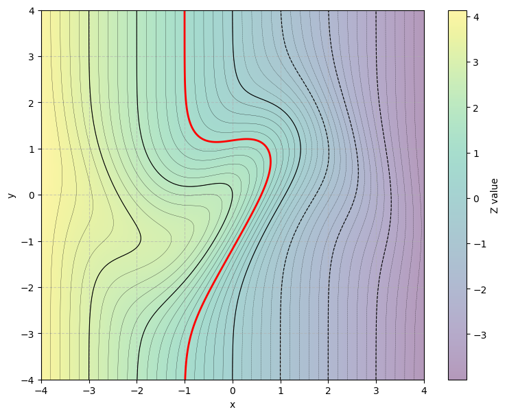
In general, if we define a random variable, $G = g(X,Y)$ , then the set of $[X,Y]$ where $G = c$ will correspond to a level set of $g$ . If $g$ is some smooth, scalar-valued function, then its level sets are usually manifolds, or unions of finitely many manifolds. To find the distribution of $G$ we will either need to find its mass function, density function, or cumulative distribution function. In each case, we will want to understand the chance that $G = c$ , or $G \leq c$ . These chances will require integrating or summing over the level sets of $g$ . Thus, they will usually require integrating or summing over some collection of manifolds.

The figure below shows an example manifold in red. It is produced by taking a level set of a scalar valued function of $x$ and $y$ (shown as contours in black with a heatmap to illustrate the function value).

Sums of Random Variables¶

Suppose that $X$ and $Y$ are jointly distributed, discrete random variables. Let $S = X + Y$ . What is $\text{PMF}_S(s) = \text{Pr}(S = s)$ ?

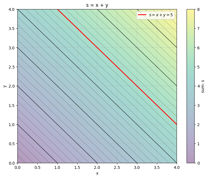
Consider all the pairs $[X,Y]$ such that $S = s$ . Since $S = X + Y$ , the collection of all pairs $[X,Y]$ such that $S = s$ is the set where $Y = s - X$ . The figure below shows, in red, the set of all $x$ and $y$ such that $s = x + y = 5$ if $x \in [0,4]$ and $y \in [0,4]$ . Notice that, the manifold corresponds to the line $y = 5 - x$ , and is a level set of the scalar valued function $x + y$ .

So, to find the chance that $S = s$ , we should take a union over all pairs of the form $[X = x, Y = s - x]$ . Since this union runs over distinct $x$ we can use additivity:

We’ve run calculations like this before (see Section 2.1). For example, suppose that you roll two fair, six-sided, die. Let $X$ and $Y$ denote the values rolled on each die. Let $S = X + Y$ . How is $S$ distributed? Try to find the distribution of $S$ yourself using a joint distribution table. Then, open the dropdown below

Solution

Suppose that you roll two fair die, and the die are distinguishable. Then there are 36 possible joint outcomes, and the joint events table is:

Roll	1	2	3	4	5	6
1	(1,1)	(1,2)	(1,3)	(1,4)	(1,5)	(1,6)
2	(2,1)	(2,2)	(2,3)	(2,4)	(2,5)	(2,6)
3	(3,1)	(3,2)	(3,3)	(3,4)	(3,5)	(3,6)
4	(4,1)	(4,2)	(4,3)	(4,4)	(4,5)	(4,6)
5	(5,1)	(5,2)	(5,3)	(5,4)	(5,5)	(5,6)
6	(6,1)	(6,2)	(6,3)	(6,4)	(6,5)	(6,6)

All 36 possible outcomes $\omega$ are equally likely since the die are fair.

Now suppose that, as is true for many games, you are interested in the sum of the rolls. Let $S(\cdot)$ denote the function that accepts an outcome $\omega$ and returns the associated sum of rolls.

Anytime you consider a random variable you should first specify its support. At least, we roll two ones. At most, we roll two sixes. So, $S \in \{1,2,3,...,11,12\}$ .

Let’s fill in the table, replacing the outcomes, $\omega$ with the sum of the rolls:

Roll	1	2	3	4	5	6
1	2	3	4	5	6	7
2	3	4	5	6	7	8
3	4	5	6	7	8	9
4	5	6	7	8	9	10
5	6	7	8	9	10	11
6	7	8	9	10	11	12

Notice that, even though all pairs of rolls were equally likely, the number of ways the pairs can add up to some value $s \in \{1,2,..., 11,12\}$ depend on $s$ .

What’s the chance that $S = 5$ ?

To find the chance, use probability by proportion. First, isolate all pairs of rolls that add to five. The associated collection is a level set of the function $S(\omega)$ it is the collection $E_5 = \{\text{all } \omega \text{ such that } S(\omega) = 5\}$ . I’ve highlighted that set below:

Roll	1	2	3	4	5	6
1	.	.	.	5	.	.
2	.	.	5	.	.	.
3	.	5	.	.	.	.
4	5	.	.	.	.	.
5	.	.	.	.	.	.
6	.	.	.	.	.	.

There are four pairs of rolls that add to 5 (four outcomes in the set $E_5$ ) so:

\text{Pr}(S = 5) = \frac{|E_5|}{|\Omega|} = \frac{4}{36} = \frac{1}{9}.

(2)

We could repeat the same process for a different value. For instance, what’s the chance $S = 10$ ?

Again, isolate the corresponding level set, and count its size. That is, count the number of ways two pairs can add to 8:

Roll	1	2	3	4	5	6
1	.	.	.	.	.	.
2	.	.	.	.	.	.
3	.	.	.	.	.	.
4	.	.	.	.	.	10
5	.	.	.	.	10	.
6	.	.	.	10	.	.

There are three pairs of rolls that add to 5 (three outcomes in the set $E_{10}$ ) so:

\text{Pr}(S = 10) = \frac{|E_{10}|}{|\Omega|} = \frac{3}{36} = \frac{1}{12}.

(3)

Repeating this process for each possible value of $s$ gives:

Value $s$	2	3	4	5	6	7	8	9	10	11	12
Chance	1/36	2/36	3/36	4/36	5/36	6/36	5/36	4/36	3/36	2/36	1/36

Even though all pairs are equally likely, not all values of the random variable are equally likely. We are twice as likely to see $S = 7$ as $S = 10$ , and six times more likely to see $S = 7$ than $S = 2$ or than $S = 12$ . The middle values are more likely since there are more ways to pick a pair that add to 6 or to 7 or to 8 than to the extreme values like 2 or 12.

If $X$ and $Y$ are continuously distributed then $S$ is also continuously distributed. Its density function is also expressed as a “sum” over the line $y = s - x$ . As usual, to move from the discrete case to the continuous case, exchange a sum with an integral:

Convolution¶

If $X$ and $Y$ are independent, then their joint mass/density function factors into a product of marginals:

\begin{aligned} & \text{Pr}(X = x,Y = y) = \text{Pr}(X = x) \times \text{Pr}(Y = y) \\ & f_{X,Y}(x,y) = f_{X}(x) \times f_{Y}(y). \end{aligned}

(5)

Factoring the joint inside of a sum over a line produces a convolution:

Convolution is an essential integral operation. It is important in many image and signal processing problems (e.g. deblurring in microscopy, astronomy, or medical imaging, and low/high-pass filtering of audio). It is the key operation behind the architecture of the convolutional neural networks widely used for computer vision, automated driving, and image classification. Convolution is also important in the theories of diffusion, a wide variety of dynamical systems, and the procedures for fast multiplication that allow computers to perform algebra quickly.

Example: Sums of Independent Exponential Random Variables¶

Suppose that $X \sim \text{Exponential}(\lambda)$ and $Y \sim \text{Exponential}(\lambda)$ are independent, identically distributed, exponential random variables. Then $X \geq 0$ and $Y \geq 0$ .

Let $S = X + Y$ . Then, $S \geq 0$ since $X$ and $Y$ are nonnegative.

If $S = s$ , then $X \in [0,s]$ since, if $X > s$ then $Y = s - X$ would be negative. Therefore:

\begin{aligned} f_S(s) & = \int_{x = 0}^{s} f_X(x) f_Y(s - x)\\ & = \lambda^2 \int_{x = 0}^s e^{-\lambda x} e^{-\lambda(s - x)} dx \\ & = \lambda^2 e^{-\lambda s} \int_{x = 0}^s e^{-(\lambda - \lambda) x} dx \\ & = \lambda^2 e^{-(\lambda + \mu) x} \int_{x = 0}^s 1 dx \\ & = \lambda^2 s e^{-\lambda s}. \end{aligned}

(8)

So, $S$ is a nonnegative random variable with density function:

f_S(s) \propto s e^{-\lambda s}.

(9)

In this case $S$ is an example of a gamma random variable.

You will iterate this analysis on your homework to find the distribution of the sum of $n$ independent, identical, exponential random variables.

Interactive¶

You can visualize convolution as follows. First, fix $s$ . Then $f_Y(s - x)$ is the function $f_Y$ reflected ( $-x$ in the argument), then translated by $s$ . So, convolving $f_X$ with $f_Y$ is the same as:

Reflecting $f_Y$ .
Translating its reflection by $s$ .
Taking the product of $f_X$ with the translated, reflected density $f_Y$ .
Finding the area underneath the product by integrating over all $x$ .

Run the code cell below to experiment with the convolution of different densities. You can choose the densities $f_X$ and $f_Y$ , visualize $f_X(x)$ and $f_Y(s - x)$ for different $s$ , reveal their product, then compute the convolution by finding the area under the product. Repeating for all $s$ recovers the density function of $S$ .

%matplotlib inline
from utils_convolution import show_convolution

show_convolution()

Sums of Squares of Random Variables¶

To estimate variances we often need to understand the distribution of sums of squares. In this chapter we’ll focus on the simple case when we add the squares of two random variables. We’ll also restrict our attention to continuous random variables.

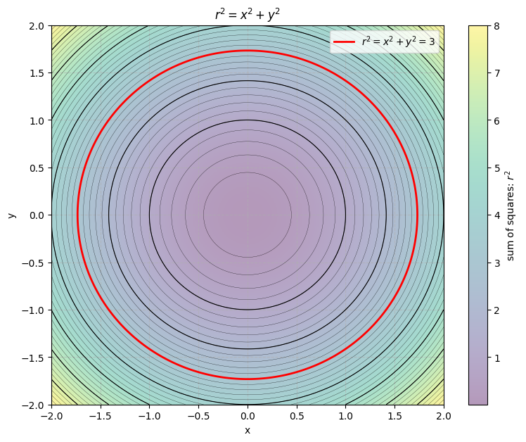
Suppose that $X$ and $Y$ are jointly distributed continuous random variables. Let $R^2 = X^2 + Y^2$ denote the sum of squares. Then, the set of all $[x,y]$ such that $x^2 + y^2 = r^2$ is a circle of radius $r$ :

How is $R^2$ distributed?

In this case it will be easier to find the distribution of $R$ by first working out its cumulative distribution function. As always, we can find its density function by differentiating its cumulative distribution function: $f_R(r) = \frac{d}{dr} F_R(r)$ (see Sections 2.3 and 2.4).

By definition,

F_R(r) = \text{Pr}(R \leq r) = \text{Pr}(R^2 \leq r^2) = \text{Pr}(X^2 + Y^2 \leq r^2).

(10)

The region where $x^2 + y^2 \leq r^2$ is the collection of all points within a circle radius $r$ , centered at the origin. So, to find the CDF of $R$ , we will need to find the volume under the joint density over the circle of radius $r$ (see Section 8.3):

F_R(r) = \iint_{[x,y] \text{ such that } x^2 + y^2 \leq r^2} f_{X,Y}(x,y) dx dy.

(11)

To integrate over a circular region, we will use an iterated integral in polar coordinates.

Integration in Polar Coordinates¶

Integration in Polar Coordinates

The double integral of a scalar valued function, $f(x,y)$ , over a region $\mathcal{R}$ , expressed in polar coordinates, is:

\iint_{[r,\theta] \text{ such that } [x,y] \in \mathcal{R}} f(r \cos(\theta), r \sin(\theta)) r dr d\theta.

(12)

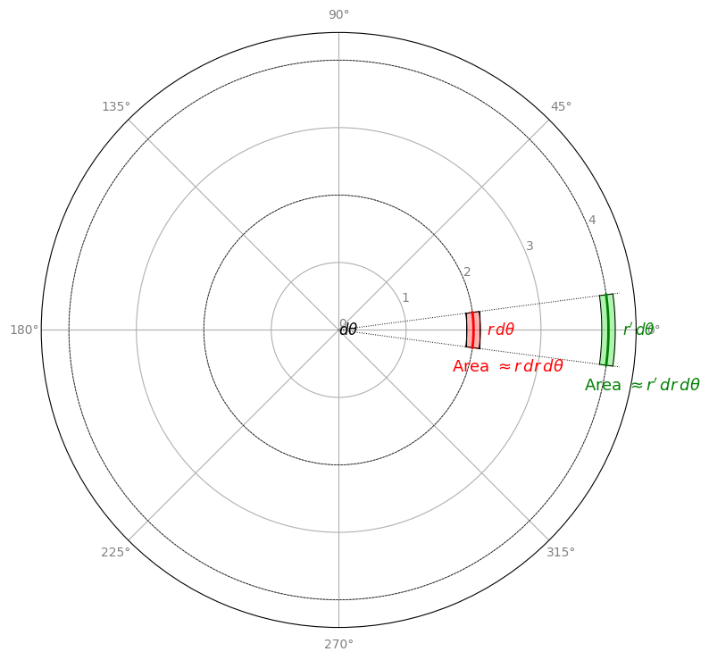
In particular, the chance that $X$ and $Y$ are contained in a circle with radius $r_*$ is:

\iint_{\text{all } x^2 + y^2 \leq r_*^2} f_{X,Y}(x,y) dx dy = \int_{r = 0}^{r_*} \left[\int_{\theta = 0}^{2 \pi} f_{X,Y}(r \cos(\theta), r \sin(\theta)) d\theta \right] r dr.

(13)

The integrand, $f$ , is usually simpler in polar coordinates if it is only a function of $r$ . If $f_{X,Y}(x,y) = g(r)$ for some nonnegative function $g$ , and $r = \sqrt{x^2 + y^2}$ , then the density is rotationally symmetric.

The integral of a rotationally symmetric density, $f_{X,Y}(x,y) = g(r)$ , over a circular region, is:

\begin{aligned} \iint_{\text{all } x^2 + y^2 \leq r_*^2} f_{X,Y}(x,y) dx dy & = \int_{r = 0}^{r_*} \left[\int_{\theta = 0}^{2 \pi} g(r) d\theta \right] r dr \\ & = \int_{r = 0}^{r_*} g(r) \left[\int_{\theta = 0}^{2 \pi} 1 d\theta \right] r dr & = 2 \pi \int_{r = 0}^{r_*} g(r) r dr. \end{aligned}

(14)

This is a univariate integral in $r$ alone.

Example: Independent Normal Random Variables¶

Suppose that $X$ and $Y$ are independent, identically distributed, standard normal random variables. Then both $X$ and $Y$ are supported on $(-\infty, \infty)$ with density function:

f_X(z) = f_Y(z) \propto e^{-\frac{1}{2} z^2}.

(15)

Since $X$ and $Y$ are independent, the random vector, $[X,Y]$ , has joint density:

f_{X,Y}(x,y) = f_X(x) \times f_Y(y) \propto e^{-\frac{1}{2}(x^2 + y^2)} = g(r)

(16)

where:

g(r) = e^{-\frac{1}{2} r^2}.

(17)

So, the joint density of $X$ and $Y$ is rotationally symmetric!

To check our work, run the code cell below and select “Independent Normal.” You should see a bell shaped peak, with circular level sets. The surface is unchanged when you rotate it, so is rotatiopnally symmetric.

from utils_lsg import show_level_sets

show_level_sets()

Let’s find the distribution of $R^2 = X^2 + Y^2$ and $R = \sqrt{X^2 + Y^2}$ . Along the way we’ll work out the normalizing constant for a single standard normal random variable.

Let’s find the distribution of $R^2$ and $R$ first. Both can be recovered from the CDF:

F_{R^2}(r_*^2) = \text{Pr}(R^2 \leq r_*^2) = \text{Pr}(R \leq r_*) = F_R(r_*).

(18)

The CDF evaluated at $r_*$ is the volume under the joint density of $X$ and $Y$ over the circle with radius $r_*$ . Integrating in polar coordinates:

F_R(r_*) \propto 2 \pi \int_{r = 0}^{r_*} g(r) r dr = 2 \pi \int_{r = 0}^{r_*} r e^{-\frac{1}{2} r^2} dr.

(19)

To evaluate the integral, let’s integrate by change of variables (see Section 7.2). Let $u = \frac{1}{2}r^2$ so that $du = (\frac{d}{dr} \frac{1}{2} r^2) dr = r dr$ . Then:

\begin{aligned} F_R(r_*) & \propto 2 \pi \int_{u = 0}^{\frac{1}{2} r_*^2} e^{-u} du \\ & = - 2 \pi e^{-u} \Big|_{u = 0}^{\frac{1}{2} r_*^2} = 2 \pi (1 - e^{-\frac{1}{2} r_*^2}).\end{aligned}

(20)

It follows that:

F_R(r) = 2 \pi c (1 - e^{-\frac{1}{2} r^2})

(21)

for some normalization constant $c$ .

To find the normalization constant, recall that $\lim_{r \rightarrow \infty} F_R(r) = 1$ for any CDF. When $r$ diverges, $r^2$ diverges, so $e^{-\frac{1}{2} r^2}$ converges to zero. Therefore:

1 = \lim_{r \rightarrow \infty} F_R(r) = 2 \pi c(1 - 0) = 2 \pi c.

(22)

Therefore, $c = 1/(2 \pi)$ .

So:

F_R(r) = 1 - e^{-\frac{1}{2} r^2}.

(23)

It follows that:

f_R(r) = \frac{d}{dr} F_R(r) = r e^{-\frac{1}{2} r^2}.

(24)

So, $R$ is a nonnegative random variable with density $f_R(r) = r e^{-\frac{1}{2} r^2}$ . In this case, $R$ is an example of a chi-squared random variable with two degrees of freedom.

To find the distribution of the sum of squares, apply the change of density formula using $y = h(r) = r^2$ (see Section 7.2). Then $h'(r) = 2 r$ and $h^{-1}(y) = \sqrt{y} = r$ . Therefore:

\begin{aligned} f_R^2(y) & = r e^{-\frac{1}{2} r^2} \frac{1}{2r} = \frac{1}{2} \frac{r}{r} e^{-\frac{1}{2} r^2} \\& = \frac{1}{2} e^{-\frac{1}{2} r^2} = \frac{1}{2} e^{-\frac{1}{2} (\sqrt{y})^2} = \frac{1}{2} e^{-\frac{1}{2} y}. \end{aligned}

(25)

So, the sum of squares, $R^2$ , is a nonnegative random variable with density proportional to an exponential function. It follows that the sum of squares is an exponential random variable with rate parameter $1/2$ .

Look back to the stage in this analysis where we worked out the normalization factor $c$ . This is the normalization factor for the joint density:

f_{X,Y}(x,y) = c g(r) = c e^{-\frac{1}{2} (x^2 + y^2)}.

(26)

Since $X$ and $Y$ are independent, with marginals, $f_X(z) = f_Y(z) \propto e^{-\frac{1}{2}z^2}$ :

\begin{aligned} f_{X,Y}(x,y) = c g(r) &= c e^{-\frac{1}{2} x^2} e^{-\frac{1}{2} y^2} \\ & = (\sqrt{c} e^{-\frac{1}{2} x^2}) (\sqrt{c} e^{-\frac{1}{2} y^2}) \\ & = f_X(x) f_Y(y). \end{aligned}.

(27)

So, the normalizing constants for the marginal densities is: $\sqrt{c} = 1/\sqrt{2 \pi}$ . Therefore, the standard normal density is normalized by:

f_Z(z) = \frac{1}{\sqrt{2 \pi}} e^{-\frac{1}{2} z^2}.

(28)

This argument explains the factor of $\sqrt{2 \pi}$ in the definition of the normal density.