10.2 Conditional and Iterated Expectation

In the last chapter we saw that double integrals and double sums can be expanded as iterated integrals and iterated sums. Since expectations are weighted averages, expectations involving two or more random variables may be expanded as multiple integrals or multiple sums. In each case, converting from a multiple integral to an iterated integral, will convert a single expectation into a pair of nested expectations.

This approach is very useful in applied problems. It breaks a problem involving two (or more) random variables into a sequence of problems, each involving only one variable at a time.

In order to understand the nested expectations, we will need to understand expectations over a single variable, fixing a different variable. An expectation given a fixed condition on some of the random inputs is a conditional expectation.

Conditional Expectation¶

Suppose that $X$ and $Y$ are jointly distributed random variables and $g(X,Y)$ is a scalar-valued function of $X$ and $Y$. Then, the conditional expectation of $g(X,Y)$ is the expected value of $g(X,Y)$ given some constraint on the values of $X$ and/or $Y$.

Applying the division rule; conditional equals joint over marginal (see Section 1.5 and Section 8.3):

Recall that, all expectations are the center of mass of some distribution (see Section 4.1). So, we can visualize the conditional expectation of $Y$ as the center of mass of the conditional distribution of $Y$ given $X = x$. Since conditional distributions are proportional to cross-sections of joint distributions (see Section 8.3), we can imagine conditional expectations as the center of mass of a cross-section of a joint.

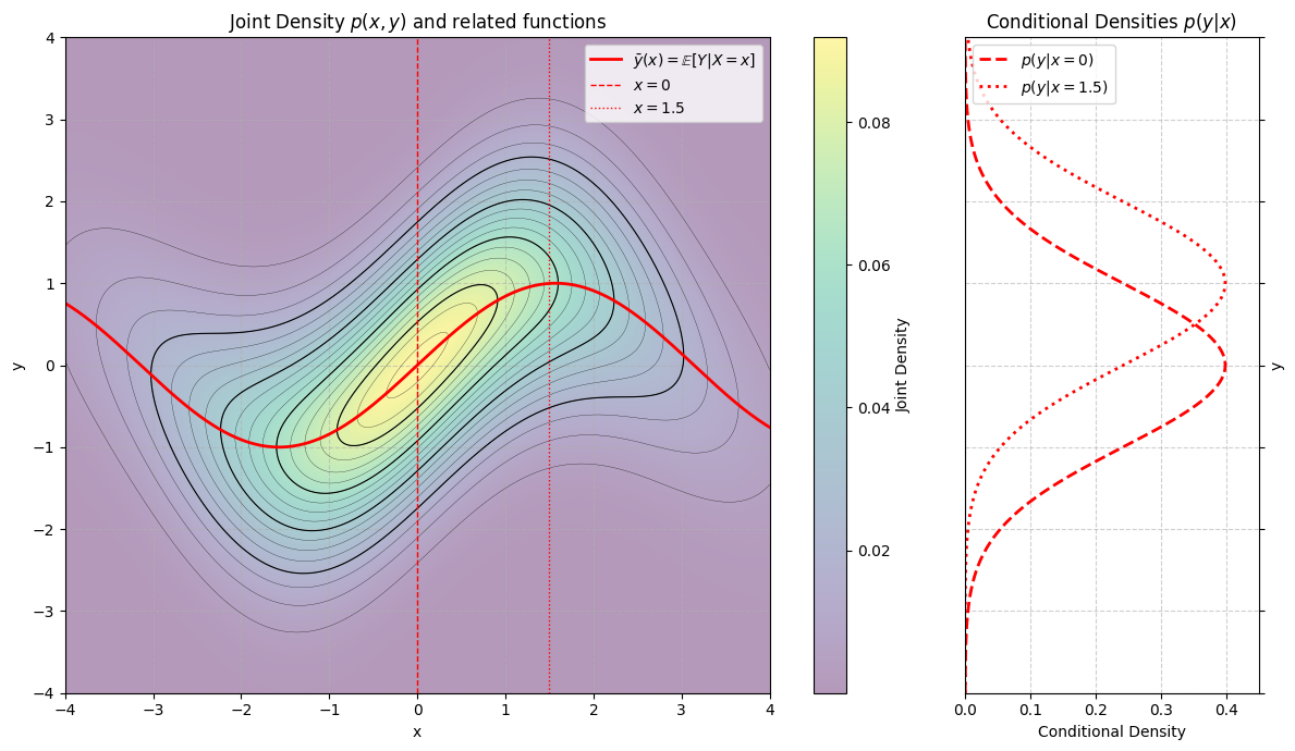
The figure below shows an example joint density function as a heat map. The contours are level sets of the density. The solid red line shows $\bar{y}(x)$, the conditional expectation of $Y$ given $X = x$. The vertical dashed and dotted red lines show the range of possible $Y$ for $X = 0$ and $X = 1.5$. The conditional distributions $f_{Y|X = 0}$ and $f_{Y|X = 1.5}$ are shown in the panel to the right. Notice that, the center of the conditionals matches the $y$-coordinate where the solid red line intersects the vertical red lines.

Run the code cell below for an interactive example. You can vary the value of $x$, and track how both the conditional distribution of $Y$ and its expectation vary as a function of $x$. Notice that the conditional density of $Y|X = x$ is proportional to the $y$-cross section of the joint density shown in the left-hand panel.

In both examples the conditional expectation of $Y$ given $X = x$ depends on the choice of $x$. This should not be surprising. The conditional distribution of $Y$ given $X = x$ is proportional to the $y$-cross-section at $x$. The $y$-cross-section varies depending on the choice of $x$, so the conditional expectation of $Y$ given $X = x$ may also vary with $x$.

Iterated Expectation¶

Iterated expectation expresses a joint expectation over both $X$ and $Y$ as an iterated expectation, first over $Y$ given $X$, then over $X$. As usual, we can choose whether to work over $X$ on the outside and $Y$ on the inside, or $Y$ on the outside and $X$ on the inside.

Loosely, you can remember this law as expressing a joint average as an average of conditional averages. Or, more succinctly, as an average of averages.

Examples¶

Like the other algebraic properties of expectation, applying iterated expectation can make it much easier to compute some joint expectations. Here are some example cases:

1. Suppose that $X$ and $Y$ are jointly distributed, where $\mathbb{E}[X] = 2$ and $\bar{y}(x) = \mathbb{E}[Y|X = x] = 4 x - 3$. What is $\mathbb{E}[Y]$?

   Solution

   Apply iterated expectation:

   $$\mathbb{E}[Y] = \mathbb{E}_{X}[\mathbb{E}_{Y|X}[Y]]] = \mathbb{E}_{X}[\bar{y}(X)] = \mathbb{E}_{X}[4 X - 3].$$

   (19)

   Then, by the linearity of expectation (see Section 4.2):

   $$\mathbb{E}[Y] = 4 \mathbb{E}[X] - 3 = 4 \times 2 - 3 = 5.$$

   (20)

   Notice that, in this example, we were able to compute the expectations without evaluating a single sum or integral. We didn’t even need to know the joint distribution!

2. Suppose that $I$ and $S$ are drawn sequentially. Suppose that $I \sim \text{Bernoulli}(1/3)$ is an indicator variable. If $I = 0$, draw $S$ from a binomial on 100 trials with success probability $1/5$. If $I = 1$, draw $S$ from a binomial on 100 trials with success probability $3/5$. Then:

   $$S|I = i \sim \begin{cases} \text{Binomial}(100,1/5) & \text{ if } i = 0 \\ \text{Binomial}(100,3/5) & \text{ if } i = 1 \\ \end{cases}$$

   (21)

   What is $\mathbb{E}[S]$?

   Solution

   Apply iterated expectation. In general, if two variables are drawn in sequence, apply iterated expectation in the same order that you would use to sample the variables:

   $$\mathbb{E}[S] = \mathbb{E}_I[\mathbb{E}_{S|I}[S]] = \sum_{i=0}^1 \bar{s}(i) \text{Pr}(I = i).$$

   (22)

   Plugging in:

   $$\mathbb{E}[S] = \bar{s}(0) \times \frac{2}{3} + \bar{s}(1) \times \frac{1}{3}.$$

   (23)

   The conditional expectations, $\bar{s}(i)$ are the expectations of binomial distributions. The expectation of a binomial equals the number of trials times the success probability. So:

   $$\bar{s}(0) = 100 \times \frac{1}{5} = 20, \quad \bar{s}(1) = 100 \times \frac{3}{5} = 60.$$

   (24)

   Therefore:

   $$\mathbb{E}[S] = \frac{2}{3} \times 20 + \frac{1}{3} \times 60 = \frac{100}{3} \approx 33.333...$$

   (25)

   In this case, the average of averages interpretation is quite clear. The values 20 and 60 are the conditional averages. The joint average is a weighted average of the conditional averages.

3. Suppose that $W \sim \text{Geometric}(p)$. What is $\mathbb{E}[W]$?

   Solution

   This doesn’t look like an obvious case for iterated integration. We computed this expectation in Section 7.1 using the tail sum formula (summation by parts). Recall that:

   $$\mathbb{E}[W] = 1/p.$$

   (26)

   This answer makes intuitive sense. A geometric random variable represents the number of trials, in a sequence of independent and identical binary trials, up to and including the first success (see Section 2.2). The parameter $p$ was the success probability. The larger $p$, the more likely each trial is to succeed, so the fewer trials needed, on average, before a success. If $p = 1/10$, then it will take 10 trials, on average, before the first success.

   Imagine running the process that produces a geometric random variable. Before you run any trials, $\mathbb{E}[W]$ represents how many trials you should expect to run before stopping.

   Now you run a trial. It either succeeds or fails. Let $I = 0$ if it fails and $I = 1$ if it succeeds. If the trial succeeds, then you stop, and $W = 1$. If it fails, you go on to the next trial.

   So, by iterated expectation:

   $$\mathbb{E}[W] = \mathbb{E}_I[\mathbb{E}_{W|I}[W]] = \text{Pr}(I = 0) \times \mathbb{E}[W|I = 0] + \text{Pr}(I = 1) \times \mathbb{E}[W|I = 1].$$

   (27)

   Substituting in the chance of success:

   $$\mathbb{E}[W] = (1 - p) \times \mathbb{E}[W|I = 0] + p \times \mathbb{E}[W|I = 1].$$

   (28)

   Since we stop immediately if we succeed, $\mathbb{E}[W|I = 1] = 1$. So:

   $$\mathbb{E}[W] = (1 - p) \times \mathbb{E}[W|I = 0] + p \times 1.$$

   (29)

   All that remains is the expected number of turns until our first sucess given that we failed on the first trial ($I = 0$). Since the trials are independent and identical, the expected additional number of trials needed to stop after failing on the first trial equals the expected number of trials needed to stop before we ran the first trial. In essence, everytime we fail, we start the process over.

   So:

   $$\times \mathbb{E}[W|I = 0] = 1 + \mathbb{E}[W].$$

   (30)

   The “1” represents the first trial that failed. The remaining $\mathbb{E}[W]$ represents the expected number of future trials until a success. Now:

   $$\mathbb{E}[W] = (1 - p) \times (1 + \mathbb{E}[W]) + p = 1 + (1 -p) \mathbb{E}[W].$$

   (31)

   Rearrange, and solve for $\mathbb{E}[W]$:

   $$(1 - (1 - p)) \mathbb{E}[W] = p \mathbb{E}[W] = 1.$$

   (32)

   Therefore:

   $$\mathbb{E}[W] = 1/p.$$

   (33)

Independent Products¶

We can use iterated expectation to prove one last property of expectations. In Section 4.2 we worked out rules for simplifying expectations of sums. We can now simplify expectations of some (not all) products: