10.1 Iterated Integrals and Sums

Iterated Integration¶

Consider a pair of variables $[x,y]$. Suppose that $f(x,y)$ is a surface. Then, the volume beneath the surface over a region $\mathcal{R}$ is defined by the double integral:

In Section 8.3 we saw that, if $f_{X,Y}$ is a density function for a random vector with two entries, then the chance a random vector falls in some region is defined as a double integral. Similarly, the expected value of a function of a random vector is defined as a double integral. In particular:

These observations generalize to more variables. For example, the chance a random vector with three entries lands in some region is expressed as a triple integral. In this chapter we will focus on the two-dimensional case. All results generalize directly to higher dimensions.

The uniform example worked above provides our first solution to a double integral.

You can compare this result to the same statement in one dimension. In one dimension, the integral of a constant over the interval is the constant times the length of the interval.

The same rule applies for double sums. The double sum of a constant equals the constant times the total number of possible index pairs used in the sum.

To evaluate general double integrals we use iterated integration.

Geometrically, iterated integration finds the volume beneath a surface by cutting the surface into cross-sections, evaluating the area under each cross-section then integrating the areas.

Note, we get to choose which variable to integrate over first. We can either integrate over $y$, then over $x$, or over $x$, then over $y$. This is an imprecise statement of Fubini’s Theorem. We won’t study the theorem formally in this class, but will use the result.

Usually we evaluate a double integral in three steps:

1. Pick an order. Choose the order so that the inner integral is easy to evaluate.

2. Suppose we chose to integrate over $y$ first. Then, let $\mathcal{R}(x)$ denote the set of all $y$ such that $[x,y] \in \mathcal{R}$. You can picture $\mathcal{R}(x_*)$ as the interval formed by drawing the intersection of $\mathcal{R}$ with the vertical line at $x = x_*$. Evaluate:

   $$A(x) = \int_{y \in \mathcal{R}(x)} f(x,y) dy$$

   (11)

   to find the area of the $y$-cross section of $f$, over $\mathcal{R}$, at $x$.

3. Integrate over $x$:

   $$\iint_{[x,y] \in \mathcal{R}} f(x,y) dx dy = \int_{x \in \mathcal{R}} A(x) dx.$$

   (12)

Notice that, by iterating, we convert a single integration problem over two variables into a sequence of two integration problems, each with respect to a single variable. To evaluate each single integral, we can use any of the techniques we’ve learned before for integration of a univariate function.

Rectangular Regions¶

Suppose that $\mathcal{R}$ is a rectangle. Then $\mathcal{R} = \{x \in [a,b], y \in [c,d]\}$ for some $a \leq b$ and some $c \leq d$. Often, rectangles are denoted using the shorthand, $\mathcal{R} = [a,b] \times [c,d]$.

If $\mathcal{R}$ is a rectangle, then the range of available $y$ is $[c,d]$, no matter $x$. Similarly, the range of available $x$ is $[a,b]$, no matter $y$. So, the double integral can be expanded:

Run the code cell below to visualize a joint density surface as a three-D histogram. It will open the same demo we used in Section 8.3.

To help visualize this volume, try running the code cell below. Pick $n = 10$. Then select “3D Perspective” and “Normalize by area”. Then, select the rectangular region $\mathcal{R} = \{x \in [0.20,0.50], y \in [0,1]\}$. You will see your rectangle highlighted with red boundaries.

Read the volume reported in the blue box at the bottom. Record the value.

Next, repeat the same experiment, computing the volumes for $x \in [0.20,0.30]$, then for $x \in [0.30, 0.40]$, then for $x \in [0.40, 0.50]$. Record each reported volume. Notice that each volume is the volume under a $y$-cross-section of the histogram.

Add up your three volumes. They will return the volume your originally computed for $x \in [0.20,0.50]$. This should be no surprise. The original volume was equal to the sum of the volume under every highlighted histogram bar. By adding over $y$ with $x$ fixed, then over $x$, you add over all the histogram bars.

This same logic applies no matter how small we make the boxes. It explains the iterated integral formula. Iterated integration is the same process we repeated above, in the limit as $n$ goes to infinity.

Try making $n$ large now. The reported volume is still the sum of the volume under each bar, and the collection of bars can still be added by first summing over $y$ fixing $x$, then over $x$.

Examples¶

1. Consider the function $f(x,y) = y (1 - (x + y))$. Let’s integrate it over $[0,0.25] \times [0,0.5]$. First, apply iterated integration:

   $$\begin{aligned} \iint_{[x,y] \in [0,0.25] \times [0,0.5]} y (1 - (x + y)) dx dy & = \int_{x = 0}^{0.25} \left( \int_{y = 0}^{0.5} y (1 - (x + y)) dy \right) dx \end{aligned}$$

   (14)

   Next, evaluate the inner integral

   $$\begin{aligned} \int_{y = 0}^{0.5} y (1 - (x + y)) dy & = (1 - x) \int_{y = 0}^{0.5} y dy - \int_{y = 0}^{0.5} y^2 dy \\ & = (1 - x) \frac{1}{2} y^2 \Big|_{y = 0}^{0.5} - \frac{1}{3} y^3 \Big|_{y = 0}^{0.5} \\ & = (1 - x) \frac{1}{2} (0.5^2 - 0) - \frac{1}{3}(0.5^3 - 0) \\ & = \frac{1}{8}(1 - x) - \frac{1}{12} \\ & = \left(\frac{1}{8} - \frac{1}{12} \right) - \frac{1}{8} x \\ & = \frac{1}{24} - \frac{1}{8} x \\ & = \frac{1}{8} \left(\frac{1}{3} - x \right)\end{aligned}$$

   (15)

   So:

   $$A(x) = \frac{1}{8} \left(\frac{1}{3} - x \right).$$

   (16)

   Notice, the area under $y$ cross-section depends on $x$ since changing $x$ changes the cross-section.

   Finally, evaluating the outer integral:

   $$\begin{aligned} \int_{x = 0}^{0.25} A(x) dx & = \frac{1}{8} \int_{x = 0}^{0.25} \left(\frac{1}{3} - x \right) dx \\ & = \frac{1}{8} \left( \frac{1}{3} x - \frac{1}{2} x^2 \right)_{x =0}^{0.25} \\ & = \frac{1}{8} \left( \frac{1}{12} - \frac{1}{32} \right) \\ & = \frac{1}{8} \times \frac{5}{96} = \frac{5}{768} \approx 0.007 \end{aligned}$$

   (17)

2. Suppose that $[X,Y]$is a continuous random vector supported on the entire $x,y$ plane. Let $f_{X,Y}$ denote the joint density function of $X$ and $Y$. What is the chance that $X \in [1,b]$?

   We can approach this problem two ways. First, since our question only involved $X$, we can ignore $Y$, and work with the marginal density of $X$, $f_X(x)$. Then, as in Section 2.3 and Section 2.4, the chance $X$ is contained in an interval is:

   $$\text{Pr}(X \in [a,b]) = \int_{x = a}^b f_X(x) dx.$$

   (18)

   Alternately, the chance $X \in [a,b]$ is the chance $[X,Y] \in \mathcal{R}$ where $\mathcal{R}$ is the rectangle with sides $[a,b]$ and $[-\infty,\infty]$ since this rectangle places no constraints on $Y$. Then:

   $$\text{Pr}(X \in [a,b]) = \text{Pr}(X \in [a,b],Y \in (-\infty,\infty)) = \iint_{[x,y] \in \mathcal{R}}f_{X,Y}(x,y) dx dy.$$

   (19)

   Let’s check that these two answers are the same.

   Expand the double integral as an iterated integral:

   $$\iint_{[x,y] \in \mathcal{R}}f_{X,Y}(x,y) dx dy = \int_{x = a}^b \left( \int_{y = -\infty}^{\infty} f_{X,Y}(x,y) dy \right) dx.$$

   (20)

   The inner integral returns the marginal density of $X$ (see Section 8.3):

   $$\int_{y = -\infty}^{\infty} f_{X,Y}(x,y) dy = f_X(x).$$

   (21)

   So, the iterated integral is equivalent to:

   $$\int_{x = a}^b \left( \int_{y = -\infty}^{\infty} f_{X,Y}(x,y) dy \right) dx = \int_{x = a}^b f_X(x) dx.$$

   (22)

   The last integral is the integral we used originally, so our answers match!

Sums and Products¶

If $f$ can be expressed as a sum or product of univariate functions, then the double integral of $f$ over a rectangular region simplifies.

For example:

Here are two examples:

1. Suppose that $X$ and $Y$ are uniformly distributed over the rectangle $[0,1] \times [0,2]$. The rectangle has area $1 \times 2 = 2$, so the joint density equals $1/2$ everywhere inside the support. Then:

   $$\mathbb{E}[XY] = \iint_{[x,y] \in [0,1] \times [0,2]} x y f_{X,Y}(x,y) dx dy = \frac{1}{2} \iint_{[x,y] \in [0,1] \times [0,2]} x y dx dy.$$

   (33)

   Then, applying our rule for products, the double integral of the product is the product of the single integrals:

   $$\mathbb{E}[XY] = \frac{1}{2} \left(\int_{x = 0}^1 x dx \right) \times \left(\int_{y = 0}^2 y dy \right).$$

   (34)

2. Suppose that $X$ and $Y$ are independent variables. Then, as shown in Section 8.3, their joint density is the product of their marginals: $f_{X,Y}(x,y) = f_X(x) \times f_Y(y)$. So:

   $$\begin{aligned} \text{Pr}(X \in [a,b],Y \in [c,d]) & = \iint_{[x,y] \in [a,b] \times [c,d]} f_{X,Y}(x,y) dx dy \\ & = \left( \int_{x = a}^b f_X(x) dx \right) \times \left( \int_{y = c}^d f_Y(y) dy \right) \\ & = \text{Pr}(X \in [a,b]) \times \text{Pr}(Y \in [c,d]). \end{aligned}$$

   (35)

   So, the product rule for double integrals recovers the product rule for independent random variables. Joint probabilities equal the product of the corresponding marginal probabilities:

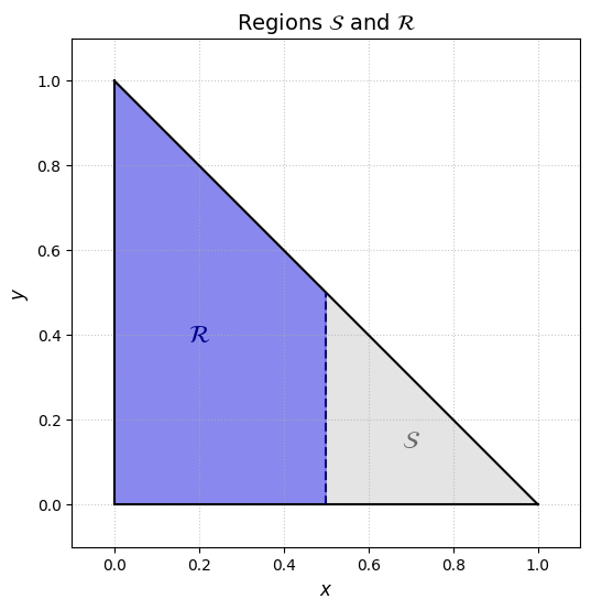
   $$\text{Pr}(X \in [a,b],Y \in [c,d]) = \text{Pr}(X \in [a,b]) \times \text{Pr}(Y \in [c,d]).$$

   (36)

Non-Rectangular Regions¶

If the region $\mathcal{R}$ is not a rectangle, then the bounds of the inner integral will depend on the outer variable. This is easiest to see by example.

Suppose that $[X,Y]$ is a random vector drawn from the region $X \geq 0$, $Y \geq 0$, $X + Y \leq 1$, with joint density:

The figure below shows the support, $\mathcal{S}$:

What is the probability that $X < 0.5?$

Let $\mathcal{R} = \{x \geq 0, y \geq 0, x + y \leq 1, x \leq 0.5 \}$. The figure below shows the region $\mathcal{R}$.

This region is a quadrilateral, with corners $\{[0,0], [0.5,0],[0,1], [0.5,0.5]\}$. It includes all $x$ between 0 and 0.5. For any $x \in [0,0.5]$ the range of available $y$ is $[0,1 - x]$ since, $x + y \leq 1$ implies $y \leq 1 - x$.

So:

Pay careful attention to the bounds of the inner integral. When $\mathcal{R}$ is not a rectangle the bounds for the inner integral will depend on the outer variable. In this case, the upper bound for $y$ depends on the choice of $x$.

To evaluate the double integral, first evaluate the inner integral:

So:

We can evaluate this integral by factoring $(1 - x)^2$ or via integration by parts (see Section 7.1). Factoring, $(1 - x)^2 = x^2 - 2 x + 1$, so:

That’s a surprisingly simple answer!

Here’s a simpler way to work it out. Recall that, finding the area under a cross-section of the joint density, over the full range of the free variable returns a marginal density (see Section 8.3):

So, in our example, $A(x) = f_X(x)$, the marginal density of $X$. Then, borrowing our previous work, the random variable $X$ is supported on $[0,1]$ with marginal density:

The function $g(x)$ is symmetric about $x = 1/2$ since it treats $x$ and $1 - x$ equivalently. Therefore, $X$ is a random variable whose distribution is even about $x = 1/2$. It follows that the chance $X < 0.5$ must match the chance $X > 0.5$. Therefore, $\text{Pr}(X \leq 0.5) = 0.5$.

Iterated Summation¶

Most integration rules also apply, by analogy, to summations. For example integrals of linear functions are linear functions of integrals. Sums of linear functions are also linear functions of sums. Integrals of products can be expanded with integration by parts. Sums of products may be expanded using summation by parts. Just as double integrals may be expanded as an iterated pair of integrals, double sums may be expanded as an iterated pair of sums.

Iterated sums expand a double sum as a sum over an outer index of a sum over an inner index, treating the outer index as if it were constant. For example, the double sum over $i$ and $j$ is the same as a sum over $i$ of a sum over $j$ given $i$.

Note that, as we saw for integrals, we can run the sum in either order. We can sum over $i$ on the outside and $j$ on the inside or $i$ on the inside and $j$ on the outside. We used this approach in Section 7.1 to derive the tail sum formula for expectations.

Here are two concrete ways to think about an iterated sum:

1. By Analogy to For Loops: If you implemented an iterated sum in code, you would use two for loops. The outer loop could run over all possible $i$. The inner loop would run over all possible $j$ given $i$.

2. By Analogy to Table Operations: Suppose you were given a table whose rows are indexed by $i$ and whose columns are indexed by $j$. Let $f(i,j)$ denote the value of the $i,j$ entry of the table. Then, a double sum over $f$ is the same as the sum of a subset of the entries of the table. Summing over $i$, then $j$ given $i$, is the same as using a sum over the columns, then a sum over the rows. Summing over $j$, then $i$ given $j$, is the same as running a sum over the rows, then a sum over the columns.

For example, suppose that $X \in \{1,2,3,4\}$ and $Y \in \{0,1,2\}$ are discrete random variables. Then we can represent their joint distribution with a joint distribution table (see Section 1.4):

Then, the probability that $X < 3$ and $Y > 0$ is the probability that $X \in [1,2]$ and $Y \in [1,2]$. Therefore:

where $\mathcal{R}$ is the rectangle $\{x \in [1,2], y \in [1,2]\}$. Excerpting the matching elements of the table:

then adding give:

Grouping terms in the sum:

is equivalent to summing across each row, then adding the row sums:

The last expression is an iterated sum.