Linear Regression - Data 89 Course Notes

Another way to summarize the relationship between two variables is by fitting one variable to a function of the other. For example, we might look for the best fit line relating $Y$ to $X$ . Then, the slope and intercept of the best fit will offer a summary of the relationship between $X$ and $Y$ . Note: we are only summarizing the relationship with the fit line, not trying to use the fit to estimate some underlying relationship.

This makes sense when the two variables satisfy a roughly linear relationship. Here’s the example we introduced in Section 10.2 again.

from utils_cond_exp import show_conditional_expectation

show_conditional_expectation()

In this case $\bar{y}(x) = \mathbb{E}[Y|X = x]$ is a linear function of $x$ , so it is very natural to summarize the relationship between $Y$ and $X$ with a line.

Finding a best fit line is an example of linear regression. We first considered linear regression in Section 9.3. We’ll recall the setting and result here, before reinterpretting the solution in terms of covariance and correlation.

Here’s an example linear regression problem using a least squares loss:

You are provided with a list of data points $\{[x_j,y_j]\}_{j=1}^n$ relating an independent variable $x$ to a dependent variable $y$ . These points form a scatter cloud in the $x, y$ plane.
You suggest a linear function that relates $x$ and $y$ , $\hat{y}(x;m,b) = m x + b$ where $m$ and $b$ are free parameters.
You aim to find the best fit function among all $\hat{y}(x;m,b)$ by minimizing some loss function that measures the discrepancy between your proposed model and the observed data:
$m*, b_* = \text{argmin}_{m,b}\{\mathcal{L}(\hat{y}(\cdot;m,b),\{[x_j,y_j]\}_{j=1}^n)\}$
(1)
It is common practice to minimize the least squares loss:
$\mathcal{L}(\hat{y}, \{[x_j,y_j]\}_{j=1}^n) = \text{MSE}(\hat{y},\{[x_j,y_j]\}_{j=1}^n) = \frac{1}{n} \sum_{j=1}^n \left(\hat{y}(x_j) - y_j \right)^2$
(2)
where $\text{MSE}$ stands for mean square error.

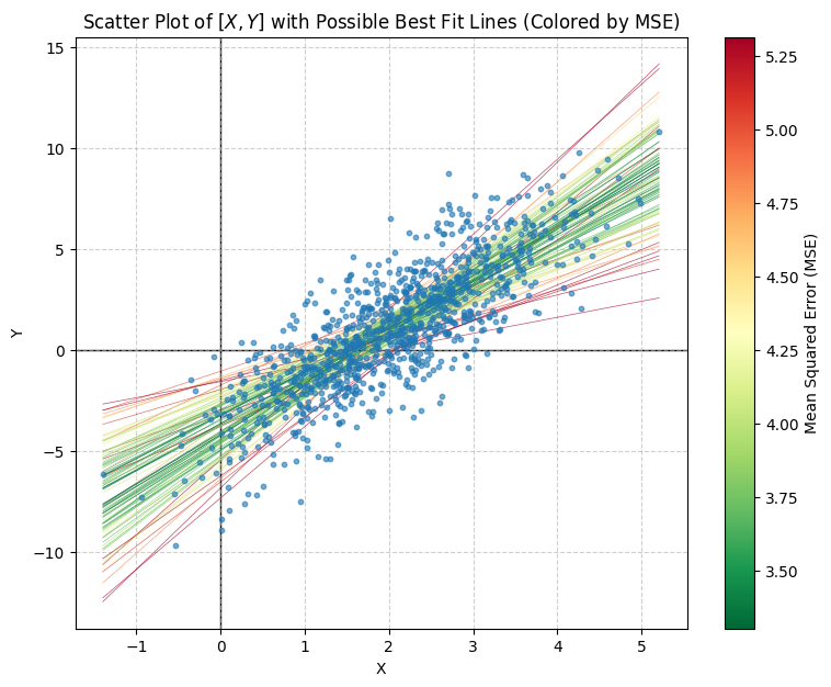
The figure below shows an example with 1000 sampled $[X,Y]$ pairs (shown as blue scatter points). The lines represent 100 possible best fit lines (produced by fitting to 100 different bootstrap samples of 10 data points). They are colored according to the quality of their fit, as measured using mean square error (the least squares loss). The lines colored red are poor fits, and produce a large loss. The lines in green are good fits, and produce a small loss. Our goal is to find a formula for the intercept and slope that minimize the loss, so provide the best summary of the relationship between $X$ and $Y$ .

Linear Least Squares Regression

The parameters $m_*,b_*$ of the linear function, $\hat{y}(x; m,b) = m x + b$ that minimize the least squares loss:

m*, b_* = \text{argmin}_{m,b}\{\frac{1}{n} \sum_{j=1}^n \left(\hat{y}(x_j;m,b) - y_j \right)^2\}

(3)

are:

b_* = -m_* \bar{x} + \bar{y}, \quad m_* = \frac{\frac{1}{n} \sum_{j=1}^n (x_j - \bar{x}) (y_j - \bar{y})}{\frac{1}{n} \sum_{j=1}^n (x_j - \bar{x})^2}

(4)

where $\bar{x} = \frac{1}{n} \sum_{j=1}^n x_j$ and $\bar{y} = \sum_{j=1}^n y_j$ are the empirical averages of the sampled $x$ ’s and $y$ ’s. Therefore, the best fit line is:

\hat{y}_*(x) = \left[\frac{\frac{1}{n} \sum_{j=1}^n (x_j - \bar{x}) (y_j - \bar{y})}{\frac{1}{n} \sum_{j=1}^n (x_j - \bar{x})^2} \right] (x - \bar{x}) + \bar{y}.

(5)

Derivation

Let $\theta = [m,b]$ denote the vector of free parameters.

To find the best fit parameters, compute the gradient of the objective, and set it equal to zero. This suffices since the objective is a convex, quadratic function of the parameters, and we’ve placed no constraints on the parameters.

\nabla_{\theta} \text{MSE}(\hat{y}(\cdot;\theta), \{[x_j,y_j]\}_{j=1}^n) = \nabla_{\theta} \frac{1}{n} \sum_{j=1}^n \left((\theta_0 + \theta_1 x_j) - y_j \right)^2

(6)

Here we’ve added the subscript $\theta$ to the gradient symbol to remind us that we are taking the gradient with respect to the parameters. Always pay careful attention to which variables you are optimizing over, and which are held fixed. In this problem the data is fixed, and we are optimizing with respect to the parameters of the model.

To compute the partial with respect to $\theta_0$ and $\theta_1$ we’ll apply the chain rule:

\begin{aligned} \partial_{\theta_i} \frac{1}{n} \sum_{j=1}^n \left((\theta_0 + \theta_1 x_j) - y_j \right)^2 & = \partial_{\theta_i} \frac{1}{n} \sum_{j=1}^n \left(\hat{y}(x_j;\theta) - y_j \right)^2 \\ & = \frac{1}{n} \sum_{j=1}^n \partial_{\theta_i} \left(\hat{y}(x_j;\theta) - y_j \right)^2 \\ & = \frac{2}{n} \sum_{j=1}^n (\hat{y}(x_j;\theta) - y_j) \times \partial_{\theta_i} \hat{y}(x_j;\theta). \end{aligned}

(7)

Then, since $\hat{y}(x;\theta) = \theta_0 + \theta_1 x$ , $\partial_{\theta_0} \hat{y}(x;\theta) = 1$ and $\partial_{\theta_1} \hat{y}(x;\theta) = x$ . So:

\nabla_{\theta} \text{MSE}(\hat{y}(\cdot;\theta), \{[x_j,y_j]\}_{j=1}^n) = \frac{2}{n} \left[ \begin{array}{c} \sum_{j=1}^n (\hat{y}(x_j;\theta) - y_j) \\ \sum_{j=1}^n (\hat{y}(x_j;\theta) - y_j) \times x_j \end{array} \right]

(8)

Setting the first entry to zero requires:

\frac{1}{n}\sum_{j=1}^n (\hat{y}(x_j;\theta_*) - y_j) = 0.

(9)

Rearranging, we need:

\frac{1}{n} \sum_{j=1}^n \hat{y}(x_j;\theta_*) = \frac{1}{n} \sum_{j=1}^n y_j = \bar{y}.

(10)

That is, the average value of the model must equal the average value of the data, $\bar{y}$ . Substituting in for $\hat{y}$ gives:

\begin{aligned} \frac{1}{n} \sum_{j=1}^n {\theta_*}_0 + {\theta_*}_1 x_j & = {\theta_*}_0 + {\theta_*}_1 \frac{1}{n} \sum_{j=1}^n x_j \\ & = {\theta_*}_0 + {\theta_*}_1 \bar{x} = \bar{y} \end{aligned}

(11)

So:

{\theta_*}_0 = \bar{y} - {\theta_*}_1 \bar{x}.

(12)

Plugging back in, we find:

\hat{y}(x;\theta_*) = \bar{y} + {\theta_*}_1 (x - \bar{x}).

(13)

This is a nicer form. It ensures that the best fit line passes through the point $[\bar{x},\bar{y}]$ where $\bar{x}$ and $\bar{y}$ are the average $x$ and $y$ coordinates in the data-set.

Now, $\hat{y}(x_j;\theta_*) - y_j$ can also be expressed more cleanly:

\hat{y}(x_j;\theta_*) - y_j = {\theta_*}_1 (x_j - \bar{x}) - (y_j - \bar{y}).

(14)

Let $x - \bar{x} = \Delta x$ and $y - \bar{y} = \Delta y$ . Then $\Delta x$ and $\Delta y$ are centered variables that represent a horizontal and vertical distance away from the mean. They correspond to the values of $x$ and $y$ had we started by centering our data (subtracting off the mean $x$ and $y$ coordinate). Many data processing pipelines start off by centering the data. Here we see a good reason to center your data when finding a best fit line. The best fit line automatically picks an intercept that effectively centers the problem. In terms of the centered variables:

\hat{y}(x_j;\theta_*) - y_j = {\theta_*}_1 \Delta x_j - \Delta y_j.

(15)

So, the second entry of the gradient can be written:

\frac{2}{n} \sum_{j=1}^n ({\theta_*}_1 \Delta x_j - \Delta y_j) \times x_j = \frac{2}{n} \sum_{j=1}^n ({\theta_*}_1 \Delta x_j - \Delta y_j) \times (\Delta x_j + \bar{x}).

(16)

The second term in the product is:

\frac{2}{n} \left[\sum_{j=1}^n ({\theta_*}_1 \Delta x_j - \Delta y_j) \right] \bar{x}.

(17)

This term is zero since we chose $\theta_*$ so that the bracketed sum equals zero. To check our work, note that:

\sum_{j=1}^n ({\theta_*}_1 \Delta x_j - \Delta y_j) = {\theta_*}_1 \sum_{j=1}^n \Delta x_j - \sum_{j=1}^n \Delta y_j ={\theta_*}_1 \times 0 - 0 = 0.

(18)

Both sums return zero since the variables $\Delta x$ and $\Delta y$ are centered.

So, the second entry in the gradient is:

\frac{2}{n} \sum_{j=1}^n ({\theta_*}_1 \Delta x_j - \Delta y_j) \times \Delta x_j.

(19)

Setting this entry to zero requires:

{\theta_*}_1 \frac{1}{n} \sum_{j=1}^n \Delta x_j^2 - \frac{1}{n} \sum_{j=1}^n \Delta y_j \Delta x_j = 0

(20)

or:

{\theta_*}_1 = \frac{\frac{1}{n} \sum_{j=1}^n \Delta y_j \Delta x_j}{\frac{1}{n} \sum_{j=1}^n \Delta x_j^2}.

(21)

Best Fit Line

Given a dataset $\{[x_j,y_j]\}_{j=1}^n$ the best fit line to the data in the least squares sense (the line that minimizes the MSE) is:

\hat{y}(x;\theta_*) = \bar{y} + {\theta_*}_1 (x - \bar{x})

(22)

where:

\begin{aligned} & \bar{x} = \frac{1}{n} \sum_{j=1}^n x_j , \quad \bar{y} = \frac{1}{n} \sum_{j=1}^n y_j \\ & {\theta_*}_1 = \frac{\frac{1}{n} \sum_{j=1}^n (y_j - \bar{y}) (x_j - \bar{x})}{\frac{1}{n} \sum_{j=1}^n (x_j - \bar{x})^2} \end{aligned}

(23)

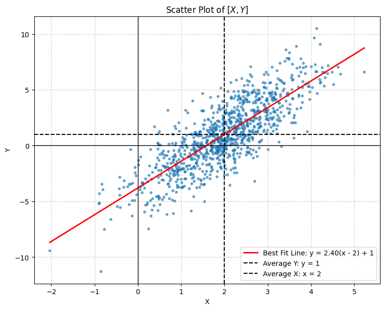
Here’s the resulting fit line (shown in red). The dashed black lines mark the empirical averages $\bar{x}$ and $\bar{y}$ .

Let’s try to make some more sense of this solution. First, since $\bar{x}$ and $\bar{y}$ are the empirical averages of the sampled $x$ ’s and $y$ ’s, if we rewtite the best fit line:

\hat{y}_*(x) - \bar{y} = m_* (x - x_*)

(24)

then we can express the best fit line in the centered coordinates:

y_0 = y - \bar{y}, \quad x_0 = x - \bar{x}, \quad {\hat{y}_0}_*(x) = m_* x_0.

(25)

This explains the best fit choice of intercept, $b_*$ . The best fit intercept is equivalent to centering the scatter cloud.

What about the best fit slope, $m_*$ ?

Consider its numerator and denominator separately:

\frac{1}{n} \sum_{j=1}^n (x_j - \bar{x}) (y_j - \bar{y}), \quad \frac{1}{n} \sum_{j=1}^n (x_j - \bar{x})^2.

(26)

These are an average product of the centered variables, and an average of the centered variables squared. In other words, the first has the form of a covariance (see Section 11.1) and the second has the form of a variance (see Section 4.3). These are the sample covariance and sample variance in the collection $\{[x_j,y_j]\}_{j=1}^n$ . They are equivalent to the covariance and variance if we choose $X$ and $Y$ by picking an index, $J$ , uniformly at random from 1 to $n$ , then setting $X = x_J$ and $Y = y_J$ . In other words:

Sample Average, Variance and Covariance

Given a collection of $n$ samples $\{[x_j,y_j]\}_{j=1}^n$ , the sample averages are:

\bar{x} = \frac{1}{n}\sum_{j=1}^n x_j, \quad \bar{y} = \frac{1}{n}\sum_{j=1}^n y_j

(27)

the sample variances are:

\frac{1}{n}\sum_{j=1}^n (x_j - \bar{x})^2, \quad \frac{1}{n}\sum_{j=1}^n (y_j - \bar{y})^2

(28)

and the sample covariance between $X$ and $Y$ is:

\frac{1}{n}\sum_{j=1}^n (x_j - \bar{x}) (y_j - \bar{y}).

(29)

The sample average, variance, and covariance, are the expected values, variances, and covariances in the random pair $[X,Y] = [x_J,Y_J]$ when $J \sim \text{Uniform}(\{1,2,3,...,n\})$ . The distribution of $[X,Y] = [x_J,Y_J]$ is the empirical distribution associated with the observed samples. So, the sample averages, variances, and covariance are the expected values, variances, and covariance in the empirical distribution.

If we use the empirical distribution, $[X,Y] = [x_J,Y_J]$ when $J \sim \text{Uniform}(\{1,2,3,...,n\})$ , then we can write:

\begin{aligned} & \bar{x} = \mathbb{E}[X], \quad \bar{y} = \mathbb{E}[Y] \\ & \text{Var}[X] = \frac{1}{n}\sum_{j=1}^n (x_j - \bar{x})^2, \quad \text{Var}[Y]= \frac{1}{n}\sum_{j=1}^n (y_j - \bar{y})^2 \\ & \text{Cov}[X,Y] = \frac{1}{n}\sum_{j=1}^n (x_j - \bar{x})^2. \end{aligned}

(30)

These equalities are exact if we use the empirical distribution. If, instead, $[X,Y]$ are drawn from the background distribution, then these equations are approximates based on the observed samples. Regardless, if $n$ is very large, then the averages associated with the background distribution, and their empirical approximations, will be very similar. Taking $n$ to infinity will drive any approximation error to zero. So, from here on out we’ll think about this result as if $X$ and $Y$ were sampled from the distribution that produced our data. We’ll study the sense in which empirical distributions and averages approximate the background distribution and averages against the background in Section 13.

We can now rephrase the best fit slope:

m_* = \frac{\text{Cov}[X,Y]}{\text{Var}[X]}

(31)

where the covariance and variance are their empirical approximations (finite $n$ ), or the true covariance and variance in $X$ and $Y$ (infinite $n$ ).

Let’s rewrite this result in terms of the correlation. Recall that:

\text{Corr}[X,Y] = \frac{\text{Cov}[X,Y]}{\text{SD}[X] \text{SD}[Y]}.

(32)

Therefore, the best fit slope is:

m_* = \frac{\text{Corr}[X,Y] \text{SD}[X] \text{SD}[Y]}{\text{Var}[X]} = \text{Corr}[X,Y] \frac{\text{SD}[Y]}{\text{SD}[X]}.

(33)

Let’s try moving all the terms involving $y$ to the left hand side. Then, the equation for the best fit line reads:

\frac{\hat{y}_*(x) - \mathbb{E}[Y]}{\text{SD}[Y]} = \text{Corr}[X,Y] \times \frac{x - \mathbb{E}[X]}{\text{SD}[X]}

(35)

The fraction on the left is the standardization of $y$ . The fraction on the right is the standardization of $x$ . So, the best fit line relating two random variables is, after standardizing, the line, passing through the origin, with slope equal to the correlation between the variables. In other words:

So, we can view the slope of a best fit line, in standard units, and correlation, as identical objects. This is useful in two ways. First, it provides an easy procedure for remembering the best fit line formula. Don’t try to memorize the messy form we found originally. Instead, do the following:

Convert to standard variables.
Set the slope of the best fit line equal to the correlation in the original variables.
Convert back as needed.

Second, it provides a clearer interpretation of the correlation and its relation to linear associations. The correlation is a slope. It is a slope in standard units. This explains both why the correlation is not a good measure for nonlinear relations, and why the correlation is a natural measure of association for variables that share a rough linear relationship. It redefines the correlation, not as an abstract measure of association, but instead as the answer to a concrete question: “what is the slope of the best fit line to this dataset/distribution?”

So, to find a correlation graphically, translate your axes to center your data. Rescale the axes so that the data cloud has the same standard deviation in each dimension. Then, estimate the slope of the best fit line. The steeper the slope, the stronger the correlation.

This interpretation also recasts the role of a best fit line. The best fit line, to a collection of data points, or a joint distribution, is, like the distribution summaries introduced in Section 4, is just another way of summarizing a distribution. It’s intercept is fixed by, and represents, the empirical averages of the data. It’s slope, after standardizing, reflects the correlation in the sampled data points!

11.2 Linear Regression