11.1 Covariance and Correlation

Objectives¶

Suppose that $X$ and $Y$ are jointly distributed random variables. How can we summarize the relationship between $X$ and $Y$ using their joint distribution? In particular, how can we summarize the degree of association between the variables?

Here’s an example. Run the code cell below. Suppose that $X$ and $Y$ were drawn from the distribution displayed. Clearly $X$ and $Y$ are related. The conditional distribution of $Y$ given $X = x$ varies as $x$ varies. Increasing $x$ increases the chance that $Y$ is large. As a result, the conditional expectation, $\bar{y}(x) = \mathbb{E}[Y|X = x]$ is an increasing function of $x$. Moreover, the conditional distribution of $Y|X = x$ is considerably narrower, for every $x$, than the marginal distribution of $Y$. That means that, if we observed $X$, we could use our observation to make better informed guesses at $Y$ than we could had we not observed $X$.

How could we summarize the strength of this relationship between $X$ and $Y$?

When defining a new mathematical object it can help to list out some desired characteristics or “desiderata”. Here are some natural desiderata for a measure of association:

It can also be helpful to identify desired “invariances”. These are ways of modifying a question that leave the answer unchanged. When measuring associations between $X$ and $Y$ there are two natural invariances:

Covariance¶

Definition¶

Let’s try to design a measure that achieves all of our desiderata.

First, let’s work out how to ensure an invariance. We’ll start with invariance to translations.

To ensure that we treat $X$ and $X + s$ the same, for all $s$, we could start by centering our random variables.

If we always start by centering our variable, then it doesn’t matter where it is centered to start. After centering it always has expectation equal to zero. So, centering will move all translations of the same distribution to the same distribution with mean zero. In particular:

for all possible $s$.

So, to ensure invariance to translations, all we have to do is start by centering our variables. If we define our measure of association using centered variables, then it will be invariant to translations.

Since we will center every variable from here on out, it will be helpful to have shorthand notation for $\mathbb{E}[X]$ and $\mathbb{E}[Y]$. We’ll use $\bar{x} = \mathbb{E}[X]$ and $\bar{y} = \mathbb{E}[Y]$.

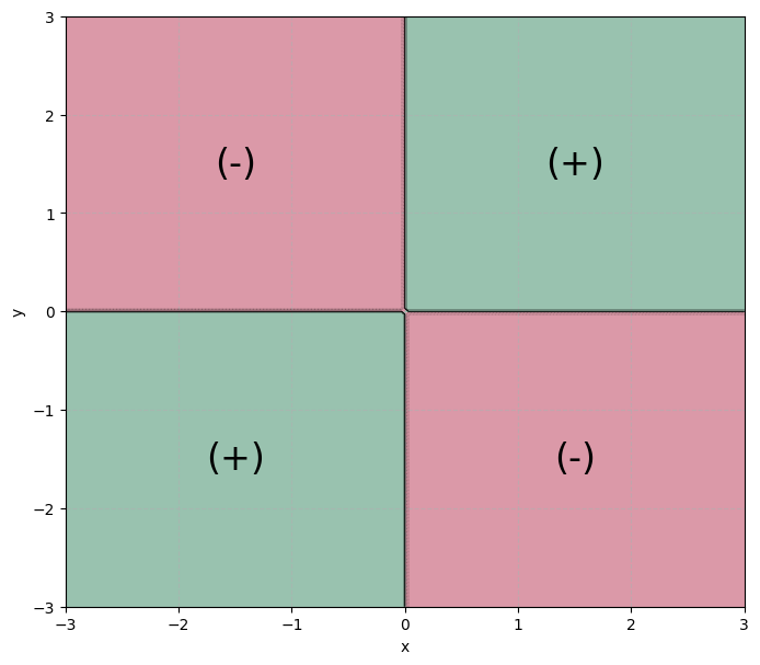
Next, let’s work on the second desiderata. Draw an $x,y$ plane. Mark the four quadrants.

Then, imagine sampling the centered variables $X_c$ and $Y_c$. The sampled pair, $[X_c,Y_c]$ could land in any of the four quadrants. If:

1. $X_0 > 0$ and $Y_0 > 0$ then both variables are larger than their expectation. This is evidence of a positive association.

2. $X_0 > 0$ and $Y_0 < 0$ then one variable is larger than its expectation and the other is smaller. This is evidence of a negative association.

3. $X_0 < 0$ and $Y_0 < 0$ then both variables are smaller than their expectation. This is evidence of a positive association.

4. $X_0 < 0$ and $Y_0 > 0$ then one variable is larger than its expectation and the other is smaller. This is evidence of a negative association.

So, imagine coloring your $x,y$ plane, using green for quadrants (I) and (III) and red for quadrants (II) and (IV). Then label the green quadrants (+) for positive association and (-) for negative association.

Let’s look for a scalar valued function of $x$ and $y$ that is positive in quadrants (I) and (III), negative in quadrants (II) and (IV), and zero on the boundaries. A natural choice is the product function $x \times y$. Notice that:

1. If $x > 0$ and $y > 0$ then $x \times y > 0$.

2. If $x > 0$ and $y < 0$ then $x \times y < 0$.

3. If $x < 0$ and $y < 0$ then $x \times y > 0$.

4. If $x < 0$ and $y > 0$ then $x \times y < 0$.

So, $x \times y$ is positive in quadrants (I) and (III), and negative in quadrants (II) and (IV). It is zero if either $x$ or $y$ are zero, so is zero along the coordinate axes dividing the quadrants. Here’s an overlaid heatmap + contour plot showing the function $x \times y$.

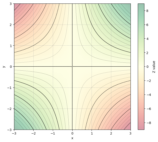
The function $x \times y$ has another useful property that aligns to our desiderata. It increases in magnitude as either input increases in magnitude. So, if $x$ is far from zero, or $y$ is far from zero, then $|x \times y|$ will be large. In contrast, if both are small, or one is much smaller than the other, then the product $|x \times y|$ will be near zero.

Since we centered our variables, the origin represents the center of mass of our distribution. So, the function $|X_c \times Y_c|$ will be large when both variables vary far from their expectations, and will be small if both stay close to their expectations.

So, the function: $X_0 \times Y_0 = (X - \bar{x}) \times (Y - \bar{y})$ is a natural measure for the degree to which a pair of sampled values jointly vary away from their expectations. In other words, it measures how much a single pair of samples “co”-vary. It is positive when the sampled vector suggests a positive association, negative when the sampled vector suggests a negative association, and is larger in magnitude the larger the variation.

Now, both samples are random, so their product, $X_0 \times Y_0$ is also a random quantity. The degree of association between two random variables should be a number determined by their joint distribution, not a number that changes depending on a particular sample. So, to average over the possible values of $X_c$ and $Y_c$, let’s use the expected value of the product as our measure of association:

The expected product of the centered variables is the covariance in $X$ and $Y$.

The covariance in $X$ and $Y$ measures how much the two variables vary together, e.g. “co”-vary. It is, by design:

1. Invariant to translations.

2. Positive when the variables are positively associated and negative when they are negatively associated.

3. Like variance, which is an expected square, the covariance, which is an expected product, is defined to give more weight to large joint variations than small variations.

Like expected values, or variances, covariances summarize an aspect of a distribution. In this case, the covariance summarizes how much the joint distribution associates positive deviations in one variable with positive deviations in the other.

Algebraic Properties of Covariance¶

Like any summary quantity defined as an expectation, the covariance has a variety of useful algebraic properties. Many of the algebraic properties of covariance are generalizations of the algebraic properties of variance. For example:

1. If either $X$ or $Y$ are constants, then the covariance in $X$ and $Y$ is zero since:

   $$\text{Cov}[c,Y] = \mathbb{E}[(c - c) \times (Y - \bar{y})] = \mathbb{E}[0 \times Y_0] = \mathbb{E}[0] = 0.$$

   (4)

   This is sensible. If one of the variables is constant, then it doesn’t vary. If one variable doesn’t vary, then the other variable can’t “co”-vary with it.

2. Covariance = expected product - product of expectations:

   $$\begin{aligned} \text{Cov}[X,Y] & = \mathbb{E}[(X - \bar{x})(Y - \bar{Y})] = \mathbb{E}[X Y - \bar{x} Y - \bar{y} X + \bar{x} \bar{y}] \\ & = \mathbb{E}[X Y] - \bar{x} \mathbb{E}[Y] - \bar{y} \mathbb{E}[X] + \bar{x} \bar{y} \\ & = \mathbb{E}[X Y] - \bar{x} \bar{y} - \bar{y} \bar{x} + \bar{x} \bar{y} \\ & = \mathbb{E}[X Y] - \bar{x} \bar{y}. \end{aligned}$$

   (5)

   So:

   $$\text{Cov}[X,Y] = \mathbb{E}[X \times Y] - \mathbb{E}[X] \times \mathbb{E}[Y].$$

   (6)

   This generalizes the formula for variance as an expected square minus a squared expectation. The covariance is the expected product minus the product of the expectations.

The algebraic properties of covariance generalize the algebraic properties of variance since variances are covariances.

So, the variance in a random variable is the covariance between the variable and itself.

Let’s check whether covariances are scale invariant:

So, covariances are not scale invariant. Instead, $\text{Cov}[a X , b Y] = ab \text{Cov}[X,Y]$. For instance, $\text{Cov}[2X, -3 Y] = -6 \text{Cov}[X,Y]$. To find a scale invariant measure of association we will need to modify the covariance to eliminate its dependence on the units of $X$ and $Y$.

Correlation¶

Definition¶

What should we do to ensure scale invariance?

Think back to how we ensured translation invariance. We started by modifying our variable. Specifically, we proposed applied a transformation to standardize some aspect of the distribution. We translated the distribution to give it a standard expectation (expectation zero).

We can generalize this standardization procedure by translating, then scaling, our random variable. We will translate to give the random variable a standard expectation (give the distribution a standard center). Then, we will scale the random variable. Scaling a random variable dilates its distribution. We will scale so that the distribution has a standard width.

Recall the following definitions from Section 4.3:

The standardized variable $Z$ is scale invariant since standardizing fixes the width of the distribution. To check, let’s standardize the variable $a X_0$:

where $Z = X_0/\text{SD}[X_0]$. So, as long as $a > 0$, the scaled variable $a X_0$ produces the same standardized variable as $X_0$.

So, to define a scale invariant measure of association, we will compute the covariance in the standardizations of $X$ and $Y$. The covariance in a standardized pair of variables is the correlation between the variables.

To compute the correlation in two random variables, standardize, then find the covariance:

so:

So, we can compute the correlation in two random variables from the covariance in the random variables and their standard deviations.

The correlation achieves all the desiderata and invariances described at the start of the chapter. Like the covariance it is translation invariant, its sign matches the sign of association, and is larger, in magnitude, the stronger the association between $X$ and $Y$. In addition, it is unitless, since standard variables are unitless. Therefore, it is scale invariant. It will not change if you change the units used to evaluate either or both random variables.

Interpretation as a Measure of Association¶

Because the correlation is unitless, and defined using standard variables, the value of the correlation can be interpreted on a standard scale.

The last point is important. It means that we can read correlation values and know immediately whether the variables are strongly or weakly associated. This is why we usually talk about the correlation between two variables, not the covariance, when we want to say they are strongly or weakly associated.

It is important that you develop an intuitive sense for large and small correlations. Navigate to this Correlation Guessing Game to practice guessing correlation values from collections of sampled $[X,Y]$ pairs.

Geometric Interpretation¶

To prove that correlations are bounded between -1 and 1, and only equal -1 or +1 in the case when $X$ and $Y$ must fall on a line, we’ll adopt a geometric interpretation of the covariance and the correlation.

First, to simplify our approach, imagine independently sampling $n$ pairs $\{[X_j,Y_j]\}_{j=1}^n$ from the joint distribution for $X$ and $Y$. Then, let $\vec{x} = [x_1,x_2,...,x_n]$ represent the vector of observed $x$ samples, and $\vec{y} = [y_1,y_2,...,y_n]$ represent the vector of observed $y$ samples. Then, we could approximate the variances and covariances needed to compute a correlation with sample averages:

where:

are the empirical averages of the sampled $X$ and $Y$ values.

These approximations are not exact, but will converge in the limit of infinite $n$. We’ll go into more detail on the convergence of sample averages to expectation in the last chapter of the book (see Section 13). For now, as we have in previous chapters, we’ll take the relation on faith.

Now, examine the empirical variances. Each is, up to scaling by $1/n$, a sum of squares of centered variables. Let $\vec{x}_0 = \vec{x} - \bar{x}$ and $\vec{y}_0 = \vec{y} - \bar{y}$ denote the centered vectors. Then, the empirical variance in the sampled $X$ values is the sum of all the entries of the centered vector, $\vec{x}_0$, squared, divided by $n$. The sum of the squares of the entries of a vector is the square of its length (see Section 8.1). So:

Therefore, the empirical standard deviations are proportional to the lengths of each vector:

Next, consider the covariance. The empirical covariance is, up to scaling by $1/n$, a sum, over every entry of $\vec{x}_0$ and $\vec{y}_0$ of the entrywise products. In other words, the empirical covariance is the inner product between $\vec{x}_0$ and $\vec{y}_0$ all divided by $n$.

So, we can estimate the correlation between $X$ and $Y$ with:

Cancelling the shared factor of $1/n$:

Recall that, the inner product between two vectors equals the products of their lengths, times the cosine of the angle between them. Therefore:

where $\theta$ is the angle between the centered vectors of sampled $X$ and centered vector of sampled $Y$. This approximation becomes exact in the limit as $n$ goes to infinity, since, as $n$ goes to infinity, each sample average converges to an expectation against the background distribution.

We can use this interpretation to show that the correlation is bounded between -1 and 1, and only equals $\pm 1$ if $X$ and $Y$ satisfy a linear relationship.

First, assume $n$ very large, so that the approximation is an equality. Then, $\text{Corr}[X,Y] = \text{cos}(\theta)$ for some angle $\theta$. The cosine of any angle is bound between -1 and 1, so $\text{Corr}[X,Y] \in [-1,1]$.

The cosine of $\theta$ only equals $\pm 1$ if $\theta = 0^{\circ}$ or $\theta = 180^{\circ}$. In other words, the cosine of the angle between two vectors is only $\pm 1$ if the vectors point in the same, or opposite directions. In either case, the vectors must be parrallel. So, $\text{Corr}[X,Y] = \pm 1$ if and only if we can guarantee that the centered vectors produced by jointly sampling $X$ and $Y$, then centering, are parallel.

This requires $\vec{x_0} \propto \vec{y}_0$ or $\vec{y}_0 = \lambda \vec{x}_0$ for some $\lambda$. Then, in terms of the original vectors of samples:

So, expanding elementwise, we need:

In other words, we need all but a vanishing fraction of the sample pairs $[x_j,y_j]$ to satisfy some linear relationship. We can only guarantee this if we can guarantee that $Y = m X + b$ for some slope and intercept $m$ and $b$ when $[X,Y]$ are drawn jointly. In other words, the correlation in $[X,Y]$ can only equal $\pm 1$ if $Y$ is a linear function of $X$.

The converse is also true. If $Y = m X + b$ for some $m$ and $b$, then the correlation equals $\pm 1$. You will check this fact on your homework.

Correlation and Dependence¶

The correlation in two variables is related to, but distinct from, the dependence or independence of the variables. Correlations look for a particular type of relationship between the variables. We will show in Section 11.2 that the correlation in two variables equals the slope of the best fit line in the standardized variables. As a result, if the variables depend on each other, but don’t share a linear relationship, they may be weakly correlated. So, weak correlations may not imply weak dependence. That said, if two variables are independent, then they cannot be correlated.

So, correlations (and covariances) satisfy the desired characteristic that, when $X$ and $Y$ are independent, the correlation and covariance in $X$ and $Y$ are both zero. It follows that, if $\text{Corr}[X,Y] \neq 0$, then $X$ and $Y$ must be dependent variables. So correlated variables are dependent.

Beware. Uncorrelated variables may also be dependent.

Here’s another example where observing $X$ would provide information about $Y$, but, the two variables don’t share a positive or negative association so are uncorrelated:

Remember: independent means uncorrelated, and correlated means dependent, but uncorrelated does not mean independent except in special cases (indicator variables or normal random variables).