13.4 The Central Limit Theorem

Motivation¶

We’ve shown that sample averages are guaranteed to converge to an underlying expectation provided the samples are sufficiently uncorrelated and are drawn with the same (or converging) expectations. We proved this result with an upper bound on tail probabilities for the distribution of the sample average. Unfortunately, the tail bounds used often overestimate the true tail probabilities. So, while strong enough to prove the weak law of large numbers, they are too weak to give useful finite sample guarantees when the user wants to guarantee accuracy with high probability.

Our results have been imprecise since we have avoided the exact distribution of the sum or sample average. This was useful since finding exact distributions is hard. We relied on summary quantites (e.g. expectations and variances) since these summaries were easier to compute and powerful enough to develop a general theory that applied no matter the original distribution. To improve on this theory we will need to study the actual distribution of long term sums and sample averages.

All examples and results in this section will pursue the exact distribution of a sum in a limit where the sum includes many terms.

Remarkably, the exact distribution of a sum, or sample average, converges, in the limit of infinitely many samples, to a normal distribution, regardless the original distribution used to generate the samples.

This theorem is the last major result in most introductory probability classes. It is especially useful when we want to produce confidence intervals. It suggests much tighter intervals than the tail bounds developed in Section 13.2. It explains the ubiquity of the normal distribution in applied probability and probability modeling.

Motivating Examples¶

To anticipate the result, we’ll consider two examples.

Bernoulli/Binomial Random Variables¶

Suppose that $\{X_j\}_{j=1}^n$ are drawn independently and identically from a Bernoulli distribution with success probability $p$.

In this case we can write down the distribution of $S_n$ exactly. The sum, $S_n = \sum_{j=1}^n I_j$, is a sum of independent, identical indicators, so is drawn from a binomial distribution with parameters $n$ and $p$:

Since we have a closed form for the PMF of the sum, we can study the limiting distribution of the sum directly. Run the code cell below to visualize the binomial distribution. Choose some $p$ and hold it fixed. Then gradually increase $n$.

You should notice three main effects:

1. As you increase $n$, the peak in the distribution slides to the right. We’ve known this for a while. The expected value of a binomial distribution is, by additivity of expectation, $n p$, and its mode is close to $n p$. So, the peak of the distribution will move rightward along the line $n p$ as a function of $n$.

2. The distribution gets wider as $n$ increases. We proved this in Section 13.1. The variance in a sum of independent, identical random variables grows proportionally to the number of terms in the sum. So, the standard deviation in $S_n$ will grow proportionally to $\sqrt{n}$. Using our rules for the variance of a sum, $\text{SD}[S_n] = \sqrt{n p (1 - p)}$.

   Notice, the standard deviation grows slower than the mean ($\mathcal{O}(n^{1/2})$ vs $\mathcal{O}(n)$). So, if your axis adjusts to fit the bulk of the distribution, the distribution may appear to grow narrower as $n$ increases. Pay attention to the marks on the $x$-axis. The distribution is getting wider as $n$ increases.

3. The distribution becomes more and more bell-shaped.

The last observation is the remarkable one. It is true for the sum of any Bernoulli random variable with $p \neq 0$ or 1. It would also be true had we used essentially any distribution to sample the $X$’s!

The function for the bell-curve you are seeing is given by the normal curve with mean $\mu = np$ and standard deviation $\sigma = \sqrt{n p (1- p)}$:

A random variable with density of the form provided above is a normal random variable. You can experiment with normal random variables by running the code cell below. Note that the normal curve has the same shape as the bell shaped histogram we observed for the binomial with large $n$.

We proved that the binomial does, in fact, converge to the normal curve at the end of Section 6.4. There, we assumed that $p = 1/2$, and proceeded with a detailed limiting analysis based on Striling’s formula (see Section 6.3).

For now, we will accept the claim based on the observation that the plotted histogram, and plotted curve, look suspiciously similar. We will recapitulate our old proof at the end of this chapter. We save the proof since the specific limiting analysis depends on details of the binomial PMF.

Our goal now is to see that we would arrive at the same normal curve, from any initial distribution. Since we can’t test all initial distributions, we’ll try a different test case.

Uniform Random Variables¶

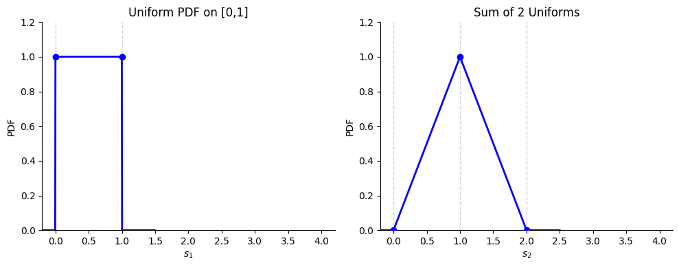
The simplest discrete case is $X_j \sim \text{Bernoulli}(0.5)$. This is a uniform distribution on the set $\{0,1\}$. Let’s try the simplest continuous analog, $X_j \sim \text{Uniform}([0,1])$. Then $X_j \in [0,1]$ for all $j$ and:

Since we’ll need this density repeatedly, let’s give it a simpler name, $f_U(x)$, where $U$ stands for uniform.

To find the density of $S_n$, work recursively:

Then, since all of the $X$’s are independent, we can derive the distribution of the sum directly by convolution (see Section 10.3):

Since the variables are identical, and uniformly distributed, we are left with the recursion:

with base case:

So, to find the density of $S_n$ we need to convolve the uniform density with itself $n$ times.

You ran the first step in discussion two weeks ago:

This density is shaped like a tent.

So, to find $S_3$, we need to compute $[f_{S_2} * f_U](s)$. Since both densities are defined piecewise, the resulting density for $S_3$ will also be defined piecwise. We can work out the boundaries between pieces as follows:

1. $S_3 < 0$ is impossible since $S_3$ is a sum of nonnegative variables.

2. $S_3 \in [0,1)$ requires $S_2 < 1$ since $X_3$ is nonnegative.

3. $S_3 \in [1,2]$ allows any $S_2 \in [0,2]$.

4. $S_3 \in (2,3]$ requires $S_2 > 1$ since $X_3$ is less than one.

5. $S_3 > 3$ is impossible since $S_3$ is a sum of three variables, all less than or equal to 1.

The first and fifth observations fix the support, $S_3 \in [0,3]$. The middle three observations divide the support into three intervals, $[0,1), [1,2], (2,3]$.

So, to find the density function, we should run convolution separately on each interval. To see the explicit convolution, open the drop down below.

After convolving, we find that $f_{S_3}(s_3)$ is a piecewise function that is:

1. zero outside $[0,3]$,

2. an upward facing parabola centered at zero connecting $(0,0)$ to $(1,1/2)$,

3. a downward facing parabola centered at 1.5 connecting $(1,1/2)$ to $(2,1/2)$,

4. then an upward facing parabola centered at 3 connecting $(2,1/2)$ to $(3,0)$.

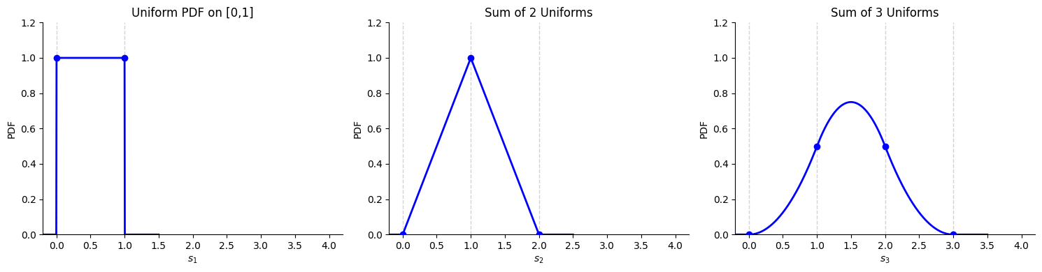
Reading in order, the density function is constant and zero, curves up, curves down, curves up, then is constant at zero again. The result is a symmetric bell centered at 1.5. The central location is sensible since $\mathbb{E}[S_3] = 3 \mathbb{E}[X_j] = 3 \times \frac{1}{2} = 1.5$.

Clearly, this procedure is too involved to continue by hand. Nevertheless, the graphical trend is clear:

1. $S_1$ is drawn from a box shaped distribution

2. $S_2$ is drawn from a tent shaped distribution

3. $S_3$ is drawn from a bell shaped distribution (with parabolic pieces)

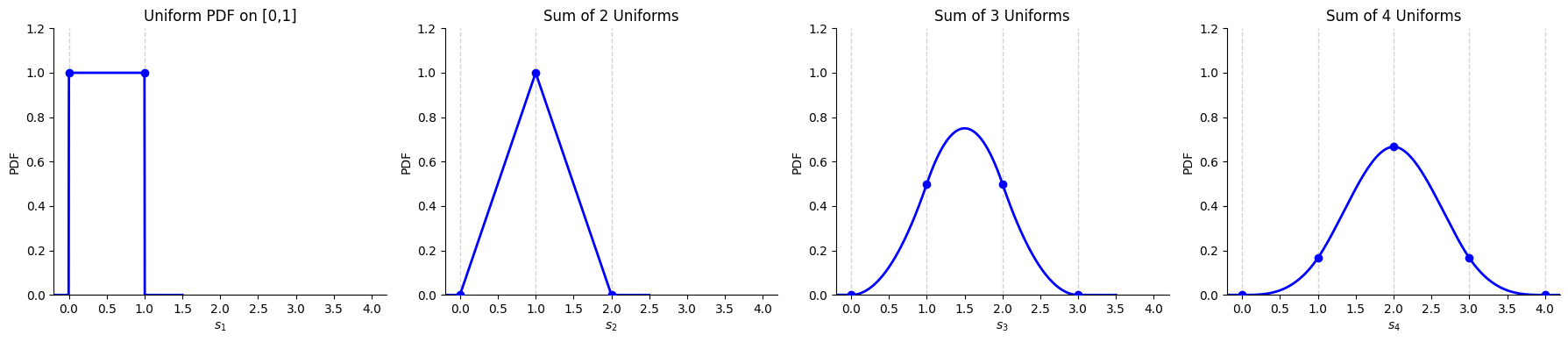
It should not be too surprising that, if we keep going, the resulting distribution becomes a smoother and smoother bell. Here are the first four densities:

The last density is very bell shaped! It is a symmetric, piecewise density, centered at 2, with three pieces, all cubic functions of $s_3$.

The limiting bell is, once again, a normal curve.

The Theorem¶

First, let’s recall the definition of a normal random variable (see Sections 5.4 and Section 6.4).

To make this statement formal, we need to adjust it in two ways. First, we need to define what we mean by convergence.

Second, we need to change to standard variables. Neither the sum, nor the sample average admit sensible limiting distributions since the expectation of the sum diverges, while the variance of the sample average converges to zero.

Go back to the binomial example. The distribution of $S_n$ slides rightward while widening as $n$ increases. So, $S_n$ doesn’t approach a random variable drawn from any fixed limiting distribution.

The sample average, $\bar{X}_n$, behaves more nicely. Its mean stays planted at $\mu$ for all $n$. However, as we increase $n$, the distribution of the sample average concentrates, so $\text{SD}[\bar{X}_n]$ converges to zero. Therefore, if $\bar{X}_n$ approaches a limiting variable, the limiting variable is deterministic, $\lim_{n \rightarrow \infty} \bar{X}_n = \mu$. So, $\bar{X}_n$ does not have an informative limiting distribution either. It’s limiting distribution has infinite density at $\mu$ and is zero everywhere else.

To get a sensible limiting distribution we need to find a transformation of $S_n$ and $\bar{X}_n$ whose mean and standard deviation converge to sensible values as $n$ diverges.

Recall that:

By construction, $Z_n$ is a standard variable, so:

Application: Frequencies Estimate Chances¶

Suppose that $\{X_j\}_{j=1}^n$ are independent, identically sampled Bernoulli random variables with unknown success probability $p$. Then, the maximum likelihood estimator for $p$ is the sample average:

The sample average is the observed frequency of success in the $n$ trials.

If $n$ is large, then $\hat{p}$ is a sample average of a large collection of independent, identical samples. So, it is approximately normally distributed with mean $\mathbb{E}[X_j] = p$ and variance $\frac{1}{n}\text{Var}[X_j] = \frac{1}{n} p (1 - p)$.

So, as long as $n$ is large, the probability that the observed frequency differs from the true success probability by more than $k$ standard deviations is, approximately:

where $Z$ is a standard normal random variable.

The probabilities that a standard normal random variable is larger, in magnitude, than an integer $k$ are well-known. We’ll compare them to the upper bounds produced by Chebyshev’s inequality (see Section 13.3)

Notice how much smaller the tail probabilities suggested by the CLT are than the upper bounds provided by Chebyshev. It follows that, when the assumptions of the CLT apply, the tail probabilities for a sample sum or sample average will often be much smaller than the Chebyshev bounds.

So, for sufficiently large $n$, the chance that the observed frequency is within 2 standard deviations of the true chance converges to about 95%, and the chance it is within three standard deviations of the mean converges to about 99.7%:

This example illustrates the power of the CLT. The CLT allows us to approximate exact tail probabilities in the limit of a large sample size, regardless the initial distribution that produces the samples! It also explains the folk wisdom, “When estimating an unknown quantity, your result is probably accurate within ± 2 standard deviations.”

Examples¶

We are not equipped to prove the CLT for arbitrary distributions. If you’d like to see the general proof, take a second course in probability (e.g. Data 140 or Stat 134).

We will satisfy ourselves with some specific cases where we can perform the limiting analysis directly. We completed the first case in Section 6.4.

Bernoulli/Binomial Random Variables¶

Let’s start with the simplest discrete example.

Suppose that $\{X_j\}_{j=1}^n \sim \text{Bernoulli}(1/2)$. Then $S_n \sim \text{Binomial}(n,1/2)$ so:

The matching standardized variable is:

The PMF of $Z_n$ is:

So, using the formula for the Binomial PMF:

To simplify, first expand the Binomial coefficient as a ratio of factorials:

Next, apply Stirling’s approximation (see Section 6.3) to approximate each term:

Substituting each term for its approximation, then cancelling like terms, gives:

When $n$ is large, $n - z^2$ will be dominated by $n$. Therefore, we can make the approximation:

The constant $2/\sqrt{n}$ out front is the interval between successive possible values of $Z_n$. We’ll call this gap $\Delta z_n$. To convert to a density function, we will divide out by $\Delta z_n$. Dividing by $\Delta z_n$ cancels the $2/\sqrt{n}$ term. For details, check the dropdown below.

Now that we’ve handled the normalizing constants, focus on the functional form:

To take the limit as $n$ goes to infinity, express each term in the form used for the limiting definition of the exponential from Section 6.2:

Therefore:

So:

The expression on the left is a PDF since $\Delta z_n$ converges to zero as $n$ diverges. The expression on the right is the standard normal density function. Therefore:

If you like challenging algebra exercises, try the same limiting analysis for generic $p$. The steps are all the same, but you will need to pay careful attention when you standardize and when you apply Striling’s formula.

Exponential Random Variables¶

Let’s try a continuous example. The uniform case is hard, so we’ll pick the next simplest example, exponential random variables.

Suppose that $\{X_j\}_{j=1}^n$ are drawn independently and identically from an exponential distribution with parameter $\lambda$.

In this case, we can work out the distribution of the sum $S_n$ exactly using convolution.

Run the code cell below to visualize the convolution of two exponential random variables. Select exponential for both distributions, then match their parameters.

The distribution you’ve produced has density function:

We proved this result in Section 10.3.

You worked out the result for general $n$ on homework 12. For the necessary work, check the matching solutions. The sum is gamma distributed with shape parameter $n$ and rate parameter $\lambda$:

Experiment with gamma distributions by running the cell below. Start with shape = 1. This returns an exponential random variable. Then increase shape to 2. This produces the gamma distribution of $S_2$. Then gradually increase the shape parameter. As you do, you will see the distribution shift to the right and become gradually more bell shaped. It remains skewed, though the skew decreases as the shape parameter increases. The mean of the distribution, which lies to the right of its mode, increases linearly in $n$.

Next, convert to a standard variable. To standardize, we need the expectation and variance in the sum. Both follow from our usual rules for expectations and variances of sums (see Section 13.1). The expectation and variance of an exponential random variable are $1/\lambda$ and $1/\lambda^2$ (see Section 7.1).

So:

To find the density function of $Z_n$, use the linear change of density formula from Section 7.2. Set $h(s) = \frac{\lambda}{\sqrt{n}} s - \sqrt{n}$. Then $h'(s) = \frac{\lambda}{\sqrt{n}}$ and $h^{-1}(z) = \frac{\sqrt{n}}{\lambda}(z + \sqrt{n})$. Then:

Simplifying:

In the limit as $n$ diverges:

Thus, the normalization constant converges to the normalization constant of the standard normal, $1/\sqrt{2 \pi}$. Open the drop-down below for the step-by-step analysis using tools from Section 6.

Now that we’ve worked out the limit of the normalization constant, we need only work out the limit of the functional form:

In this case it will be easier to work out the limit of the logarithm of the functional form. Since the log is continuous, the limit of the logarithm is the logarithm of the limit. So, we can find the original limit by taking the limit of the logarithm, then exponentiating our answer.

We can simplify the first term since $\lim_{n \rightarrow 0} z/\sqrt{n} = 0$ so:

Therefore:

Since $z/\sqrt{n}$ is small when $n$ is large, we can replace the logarithm with its Taylor expansion near zero (see Section 6.1). In this case we will need to go past our usual linear approximation to the log and include quadratic terms:

Therefore:

Multiplying by $n$:

Therefore:

Anything proportional to $n^{-1/2}$ converges to zero as $n$ diverges so:

So, working back:

This is the functional form for a standard normal density!

Putting the functional form and the normalization constant together:

where $Z$ is a standard normal variable. Therefore $\lim_{n \rightarrow \infty} Z_n = Z$, a standard normal random variable!